Lesson Template

Programming with Python

The best way to learn how to program is to do something useful, so this introduction to Python is built around a common scientific task: data analysis.

Our real goal isn't to teach you Python, but to teach you the basic concepts that all programming depends on. We use Python in our lessons because:

1. we have to use something for examples;
2. it's free, well-documented, and runs almost everywhere;
3. it has a large (and growing) user base among scientists; and
4. experience shows that it's easier for novices to pick up than most other languages.

But the two most important things are to use whatever language your colleagues are using, so that you can share your work with them easily, and to use that language well.

We are studying inflammation in patients who have been given a new treatment for arthritis, and need to analyze the first dozen data sets of their daily inflammation. The data sets are stored in comma-separated values (CSV) format: each row holds information for a single patient, and the columns represent successive days. The first few rows of our first file look like this:

0,0,1,3,1,2,4,7,8,3,3,3,10,5,7,4,7,7,12,18,6,13,11,11,7,7,4,6,8,8,4,4,5,7,3,4,2,3,0,0
0,1,2,1,2,1,3,2,2,6,10,11,5,9,4,4,7,16,8,6,18,4,12,5,12,7,11,5,11,3,3,5,4,4,5,5,1,1,0,1
0,1,1,3,3,2,6,2,5,9,5,7,4,5,4,15,5,11,9,10,19,14,12,17,7,12,11,7,4,2,10,5,4,2,2,3,2,2,1,1
0,0,2,0,4,2,2,1,6,7,10,7,9,13,8,8,15,10,10,7,17,4,4,7,6,15,6,4,9,11,3,5,6,3,3,4,2,3,2,1
0,1,1,3,3,1,3,5,2,4,4,7,6,5,3,10,8,10,6,17,9,14,9,7,13,9,12,6,7,7,9,6,3,2,2,4,2,0,1,1

We want to:

• load that data into memory,
• calculate the average inflammation per day across all patients, and
• plot the result.

To do all that, we'll have to learn a little bit about programming.

$ cd && cd Desktop/python-novice-inflammation/data

Topics

1. Analyzing Patient Data
2. Repeating Actions with Loops
3. Storing Multiple Values in Lists
4. Analyzing Data from Multiple Files
5. Making Choices
6. Creating Functions
7. Errors and Exceptions
8. Defensive Programming
9. Debugging
10. Command-Line Programs

Other Resources

• Reference
• Discussion
• Instructor's Guide

Analyzing Patient Data

Words are useful, but what's more useful are the sentences and stories we build with them. Similarly, while a lot of powerful tools are built into languages like Python, even more live in the libraries they are used to build.

In order to load our inflammation data, we need to import a library called NumPy. In general you should use this library if you want to do fancy things with numbers, especially if you have matrices or arrays. We can load NumPy using:

import numpy

Importing a library is like getting a piece of lab equipment out of a storage locker and setting it up on the bench. Once you've loaded the library, we can ask the library to read our data file for us:

numpy.loadtxt(fname='inflammation-01.csv', delimiter=',')

array([[ 0.,  0.,  1., ...,  3.,  0.,  0.],
       [ 0.,  1.,  2., ...,  1.,  0.,  1.],
       [ 0.,  1.,  1., ...,  2.,  1.,  1.],
       ...,
       [ 0.,  1.,  1., ...,  1.,  1.,  1.],
       [ 0.,  0.,  0., ...,  0.,  2.,  0.],
       [ 0.,  0.,  1., ...,  1.,  1.,  0.]])

The expression numpy.loadtxt(...) is a function call that asks Python to run the function loadtxt that belongs to the numpy library. This dotted notation is used everywhere in Python to refer to the parts of things as thing.component.

numpy.loadtxt has two parameters: the name of the file we want to read, and the delimiter that separates values on a line. These both need to be character strings (or strings for short), so we put them in quotes.

When we are finished typing and press Shift+Enter, the notebook runs our command. Since we haven't told it to do anything else with the function's output, the notebook displays it. In this case, that output is the data we just loaded. By default, only a few rows and columns are shown (with ... to omit elements when displaying big arrays). To save space, Python displays numbers as 1. instead of 1.0 when there's nothing interesting after the decimal point.

Our call to numpy.loadtxt read our file, but didn't save the data in memory. To do that, we need to assign the array to a variable. A variable is just a name for a value, such as x, current_temperature, or subject_id. Python's variables must begin with a letter and are case sensitive. We can create a new variable by assigning a value to it using =. As an illustration, let's step back and instead of considering a table of data, consider the simplest "collection" of data, a single value. The line below assigns the value 55 to a variable weight_kg:

weight_kg = 55

Once a variable has a value, we can print it to the screen:

print weight_kg

55

and do arithmetic with it:

print 'weight in pounds:', 2.2 * weight_kg

weight in pounds: 121.0

We can also change a variable's value by assigning it a new one:

weight_kg = 57.5
print 'weight in kilograms is now:', weight_kg

weight in kilograms is now: 57.5

As the example above shows, we can print several things at once by separating them with commas.

If we imagine the variable as a sticky note with a name written on it, assignment is like putting the sticky note on a particular value:

Variables as Sticky Notes

This means that assigning a value to one variable does not change the values of other variables. For example, let's store the subject's weight in pounds in a variable:

weight_lb = 2.2 * weight_kg
print 'weight in kilograms:', weight_kg, 'and in pounds:', weight_lb

weight in kilograms: 57.5 and in pounds: 126.5

Creating Another Variable

and then change weight_kg:

weight_kg = 100.0
print 'weight in kilograms is now:', weight_kg, 'and weight in pounds is still:', weight_lb

weight in kilograms is now: 100.0 and weight in pounds is still: 126.5

Updating a Variable

Since weight_lb doesn't "remember" where its value came from, it isn't automatically updated when weight_kg changes. This is different from the way spreadsheets work.

Just as we can assign a single value to a variable, we can also assign an array of values to a variable using the same syntax. Let's re-run numpy.loadtxt and save its result:

data = numpy.loadtxt(fname='inflammation-01.csv', delimiter=',')

This statement doesn't produce any output because assignment doesn't display anything. If we want to check that our data has been loaded, we can print the variable's value:

print data

[[ 0.  0.  1. ...,  3.  0.  0.]
 [ 0.  1.  2. ...,  1.  0.  1.]
 [ 0.  1.  1. ...,  2.  1.  1.]
 ...,
 [ 0.  1.  1. ...,  1.  1.  1.]
 [ 0.  0.  0. ...,  0.  2.  0.]
 [ 0.  0.  1. ...,  1.  1.  0.]]

Now that our data is in memory, we can start doing things with it. First, let's ask what type of thing data refers to:

print type(data)

<type 'numpy.ndarray'>

The output tells us that data currently refers to an N-dimensional array created by the NumPy library. These data corresponds to arthritis patient's inflammation. The rows are the individual patients and the columns are there daily inflammation measurements. We can see what its shape is like this:

print data.shape

(60, 40)

This tells us that data has 60 rows and 40 columns. When we created the variable data to store our arthritis data, we didn't just create the array, we also created information about the array, called members or attributes. This extra information describes data in the same way an adjective describes a noun. data.shape is an attribute of data which described the dimensions of data. We use the same dotted notation for the attributes of variables that we use for the functions in libraries because they have the same part-and-whole relationship.

If we want to get a single number from the array, we must provide an index in square brackets, just as we do in math:

print 'first value in data:', data[0, 0]

first value in data: 0.0

print 'middle value in data:', data[30, 20]

middle value in data: 13.0

The expression data[30, 20] may not surprise you, but data[0, 0] might. Programming languages like Fortran and MATLAB start counting at 1, because that's what human beings have done for thousands of years. Languages in the C family (including C++, Java, Perl, and Python) count from 0 because that's simpler for computers to do. As a result, if we have an M×N array in Python, its indices go from 0 to M-1 on the first axis and 0 to N-1 on the second. It takes a bit of getting used to, but one way to remember the rule is that the index is how many steps we have to take from the start to get the item we want.

An index like [30, 20] selects a single element of an array, but we can select whole sections as well. For example, we can select the first ten days (columns) of values for the first four patients (rows) like this:

print data[0:4, 0:10]

[[ 0.  0.  1.  3.  1.  2.  4.  7.  8.  3.]
 [ 0.  1.  2.  1.  2.  1.  3.  2.  2.  6.]
 [ 0.  1.  1.  3.  3.  2.  6.  2.  5.  9.]
 [ 0.  0.  2.  0.  4.  2.  2.  1.  6.  7.]]

The slice 0:4 means, "Start at index 0 and go up to, but not including, index 4." Again, the up-to-but-not-including takes a bit of getting used to, but the rule is that the difference between the upper and lower bounds is the number of values in the slice.

We don't have to start slices at 0:

print data[5:10, 0:10]

[[ 0.  0.  1.  2.  2.  4.  2.  1.  6.  4.]
 [ 0.  0.  2.  2.  4.  2.  2.  5.  5.  8.]
 [ 0.  0.  1.  2.  3.  1.  2.  3.  5.  3.]
 [ 0.  0.  0.  3.  1.  5.  6.  5.  5.  8.]
 [ 0.  1.  1.  2.  1.  3.  5.  3.  5.  8.]]

We also don't have to include the upper and lower bound on the slice. If we don't include the lower bound, Python uses 0 by default; if we don't include the upper, the slice runs to the end of the axis, and if we don't include either (i.e., if we just use ':' on its own), the slice includes everything:

small = data[:3, 36:]
print 'small is:'
print small

small is:
[[ 2.  3.  0.  0.]
 [ 1.  1.  0.  1.]
 [ 2.  2.  1.  1.]]

Arrays also know how to perform common mathematical operations on their values. The simplest operations with data are arithmetic: add, subtract, multiply, and divide. When you do such operations on arrays, the operation is done on each individual element of the array. Thus:

doubledata = data * 2.0

will create a new array doubledata whose elements have the value of two times the value of the corresponding elements in data:

print 'original:'
print data[:3, 36:]
print 'doubledata:'
print doubledata[:3, 36:]

original:
[[ 2.  3.  0.  0.]
 [ 1.  1.  0.  1.]
 [ 2.  2.  1.  1.]]
doubledata:
[[ 4.  6.  0.  0.]
 [ 2.  2.  0.  2.]
 [ 4.  4.  2.  2.]]

If, instead of taking an array and doing arithmetic with a single value (as above) you did the arithmetic operation with another array of the same shape, the operation will be done on corresponding elements of the two arrays. Thus:

tripledata = doubledata + data

will give you an array where tripledata[0,0] will equal doubledata[0,0] plus data[0,0], and so on for all other elements of the arrays.

print 'tripledata:'
print tripledata[:3, 36:]

tripledata:
[[ 6.  9.  0.  0.]
 [ 3.  3.  0.  3.]
 [ 6.  6.  3.  3.]]

Often, we want to do more than add, subtract, multiply, and divide values of data. Arrays also know how to do more complex operations on their values. If we want to find the average inflammation for all patients on all days, for example, we can just ask the array for its mean value

print data.mean()

6.14875

mean is a method of the array, i.e., a function that belongs to it in the same way that the member shape does. If variables are nouns, methods are verbs: they are what the thing in question knows how to do. We need empty parentheses for data.mean(), even when we're not passing in any parameters, to tell Python to go and do something for us. data.shape doesn't need () because it is just a description but data.mean() requires the () because it is an action.

NumPy arrays have lots of useful methods:

print 'maximum inflammation:', data.max()
print 'minimum inflammation:', data.min()
print 'standard deviation:', data.std()

maximum inflammation: 20.0
minimum inflammation: 0.0
standard deviation: 4.61383319712

When analyzing data, though, we often want to look at partial statistics, such as the maximum value per patient or the average value per day. One way to do this is to create a new temporary array of the data we want, then ask it to do the calculation:

patient_0 = data[0, :] # 0 on the first axis, everything on the second
print 'maximum inflammation for patient 0:', patient_0.max()

maximum inflammation for patient 0: 18.0

We don't actually need to store the row in a variable of its own. Instead, we can combine the selection and the method call:

print 'maximum inflammation for patient 2:', data[2, :].max()

maximum inflammation for patient 2: 19.0

What if we need the maximum inflammation for all patients (as in the next diagram on the left), or the average for each day (as in the diagram on the right)? As the diagram below shows, we want to perform the operation across an axis:

Operations Across Axes

To support this, most array methods allow us to specify the axis we want to work on. If we ask for the average across axis 0 (rows in our 2D example), we get:

print data.mean(axis=0)

[  0.           0.45         1.11666667   1.75         2.43333333   3.15
   3.8          3.88333333   5.23333333   5.51666667   5.95         5.9
   8.35         7.73333333   8.36666667   9.5          9.58333333
  10.63333333  11.56666667  12.35        13.25        11.96666667
  11.03333333  10.16666667  10.           8.66666667   9.15         7.25
   7.33333333   6.58333333   6.06666667   5.95         5.11666667   3.6
   3.3          3.56666667   2.48333333   1.5          1.13333333
   0.56666667]

As a quick check, we can ask this array what its shape is:

print data.mean(axis=0).shape

(40,)

The expression (40,) tells us we have an N×1 vector, so this is the average inflammation per day for all patients. If we average across axis 1 (columns in our 2D example), we get:

print data.mean(axis=1)

[ 5.45   5.425  6.1    5.9    5.55   6.225  5.975  6.65   6.625  6.525
  6.775  5.8    6.225  5.75   5.225  6.3    6.55   5.7    5.85   6.55
  5.775  5.825  6.175  6.1    5.8    6.425  6.05   6.025  6.175  6.55
  6.175  6.35   6.725  6.125  7.075  5.725  5.925  6.15   6.075  5.75
  5.975  5.725  6.3    5.9    6.75   5.925  7.225  6.15   5.95   6.275  5.7
  6.1    6.825  5.975  6.725  5.7    6.25   6.4    7.05   5.9  ]

which is the average inflammation per patient across all days.

The mathematician Richard Hamming once said, "The purpose of computing is insight, not numbers," and the best way to develop insight is often to visualize data. Visualization deserves an entire lecture (or course) of its own, but we can explore a few features of Python's matplotlib library here. While there is no "official" plotting library, this package is the de facto standard. First, we will import the pyplot module from matplotlib and use two of its functions to create and display a heat map of our data:

import matplotlib.pyplot
image  = matplotlib.pyplot.imshow(data)
matplotlib.pyplot.show(image)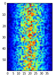

Heatmap of the Data

Blue regions in this heat map are low values, while red shows high values. As we can see, inflammation rises and falls over a 40-day period.

Let's take a look at the average inflammation over time:

ave_inflammation = data.mean(axis=0)
ave_plot = matplotlib.pyplot.plot(ave_inflammation)
matplotlib.pyplot.show(ave_plot)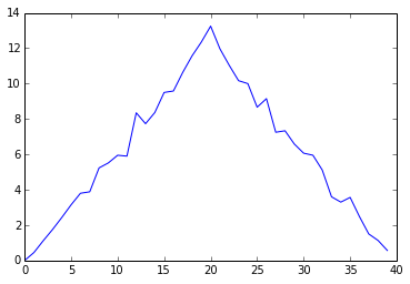

Average Inflammation Over Time

Here, we have put the average per day across all patients in the variable ave_inflammation, then asked matplotlib.pyplot to create and display a line graph of those values. The result is roughly a linear rise and fall, which is suspicious: based on other studies, we expect a sharper rise and slower fall. Let's have a look at two other statistics:

max_plot = matplotlib.pyplot.plot(data.max(axis=0))
matplotlib.pyplot.show(max_plot)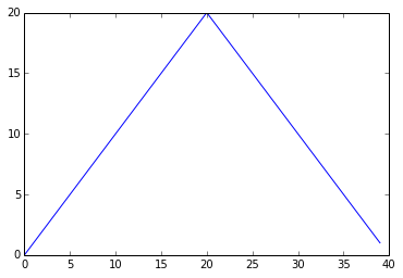

Maximum Value Along The First Axis

min_plot = matplotlib.pyplot.plot(data.min(axis=0))
matplotlib.pyplot.show(min_plot)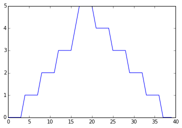

Minimum Value Along The First Axis

The maximum value rises and falls perfectly smoothly, while the minimum seems to be a step function. Neither result seems particularly likely, so either there's a mistake in our calculations or something is wrong with our data.

You can group similar plots in a single figure using subplots. This script below uses a number of new commands. The function matplotlib.pyplot.figure() creates a space into which we will place all of our plots. The parameter figsize tells Python how big to make this space. Each subplot is placed into the figure using the subplot command. The subplot command takes 3 parameters. The first denotes how many total rows of subplots there are, the second parameter refers to the total number of subplot columns, and the final parameters denotes which subplot your variable is referencing. Each subplot is stored in a different variable (axes1, axes2, axes3). Once a subplot is created, the axes are can be titled using the set_xlabel() command (or set_ylabel()). Here are our three plots side by side:

import numpy
import matplotlib.pyplot

data = numpy.loadtxt(fname='inflammation-01.csv', delimiter=',')

fig = matplotlib.pyplot.figure(figsize=(10.0, 3.0))

axes1 = fig.add_subplot(1, 3, 1)
axes2 = fig.add_subplot(1, 3, 2)
axes3 = fig.add_subplot(1, 3, 3)

axes1.set_ylabel('average')
axes1.plot(data.mean(axis=0))

axes2.set_ylabel('max')
axes2.plot(data.max(axis=0))

axes3.set_ylabel('min')
axes3.plot(data.min(axis=0))

fig.tight_layout()

matplotlib.pyplot.show(fig)

The Previous Plots as Subplots

The call to loadtxt reads our data, and the rest of the program tells the plotting library how large we want the figure to be, that we're creating three sub-plots, what to draw for each one, and that we want a tight layout. (Perversely, if we leave out that call to fig.tight_layout(), the graphs will actually be squeezed together more closely.)

mass = 47.5
age = 122
mass = mass * 2.0
age = age - 20

first, second = 'Grace', 'Hopper'
third, fourth = second, first
print third, fourth

element = 'oxygen'
print 'first three characters:', element[0:3]
print 'last three characters:', element[3:6]

first three characters: oxy
last three characters: gen

Repeating Actions with Loops

In the last lesson, we wrote some code that plots some values of interest from our first inflammation dataset, and reveals some suspicious features in it, such as from inflammation-01.csv

but we have a dozen data sets right now and more on the way. We want to create plots for all our data sets with a single statement. To do that, we'll have to teach the computer how to repeat things.

An example task that we might want to repeat is printing each character in a word on a line of its own. One way to do this would be to use a series of print statements:

word = 'lead'
print word[0]
print word[1]
print word[2]
print word[3]

l
e
a
d

but that's a bad approach for two reasons:

1. It doesn't scale: if we want to print the characters in a string that's hundreds of letters long, we'd be better off just typing them in.

2. It's fragile: if we give it a longer string, it only prints part of the data, and if we give it a shorter one, it produces an error because we're asking for characters that don't exist.

word = 'tin'
print word[0]
print word[1]
print word[2]
print word[3]

t
i
n

---------------------------------------------------------------------------
IndexError                                Traceback (most recent call last)
<ipython-input-3-7974b6cdaf14> in <module>()
      3 print word[1]
      4 print word[2]
----> 5 print word[3]

IndexError: string index out of range

Here's a better approach:

word = 'lead'
for char in word:
    print char

l
e
a
d

This is shorter---certainly shorter than something that prints every character in a hundred-letter string---and more robust as well:

word = 'oxygen'
for char in word:
    print char

o
x
y
g
e
n

The improved version of print_characters uses a for loop to repeat an operation---in this case, printing---once for each thing in a collection. The general form of a loop is:

for variable in collection:
    do things with variable

We can call the loop variable anything we like, but there must be a colon at the end of the line starting the loop, and we must indent anything we want to run inside the loop. Unlike many other languages, there is no command to end a loop (e.g. end for); what is indented after the for statement belongs to the loop.

Here's another loop that repeatedly updates a variable:

length = 0
for vowel in 'aeiou':
    length = length + 1
print 'There are', length, 'vowels'

There are 5 vowels

It's worth tracing the execution of this little program step by step. Since there are five characters in 'aeiou', the statement on line 3 will be executed five times. The first time around, length is zero (the value assigned to it on line 1) and vowel is 'a'. The statement adds 1 to the old value of length, producing 1, and updates length to refer to that new value. The next time around, vowel is 'e' and length is 1, so length is updated to be 2. After three more updates, length is 5; since there is nothing left in 'aeiou' for Python to process, the loop finishes and the print statement on line 4 tells us our final answer.

Note that a loop variable is just a variable that's being used to record progress in a loop. It still exists after the loop is over, and we can re-use variables previously defined as loop variables as well:

letter = 'z'
for letter in 'abc':
    print letter
print 'after the loop, letter is', letter

a
b
c
after the loop, letter is c

Note also that finding the length of a string is such a common operation that Python actually has a built-in function to do it called len:

print len('aeiou')

5

len is much faster than any function we could write ourselves, and much easier to read than a two-line loop; it will also give us the length of many other things that we haven't met yet, so we should always use it when we can.

1
2
3

print 5 ** 3
125

Storing Multiple Values in Lists

Just as a for loop is a way to do operations many times, a list is a way to store many values. Unlike NumPy arrays, lists are built into the language (so we don't have to load a library to use them). We create a list by putting values inside square brackets:

odds = [1, 3, 5, 7]
print 'odds are:', odds

odds are: [1, 3, 5, 7]

We select individual elements from lists by indexing them:

print 'first and last:', odds[0], odds[-1]

first and last: 1 7

and if we loop over a list, the loop variable is assigned elements one at a time:

for number in odds:
    print number

1
3
5
7

There is one important difference between lists and strings: we can change the values in a list, but we cannot change the characters in a string. For example:

names = ['Newton', 'Darwing', 'Turing'] # typo in Darwin's name
print 'names is originally:', names
names[1] = 'Darwin' # correct the name
print 'final value of names:', names

names is originally: ['Newton', 'Darwing', 'Turing']
final value of names: ['Newton', 'Darwin', 'Turing']

works, but:

name = 'Bell'
name[0] = 'b'

---------------------------------------------------------------------------
TypeError                                 Traceback (most recent call last)
<ipython-input-8-220df48aeb2e> in <module>()
      1 name = 'Bell'
----> 2 name[0] = 'b'

TypeError: 'str' object does not support item assignment

does not.

There are many ways to change the contents of lists besides assigning new values to individual elements:

odds.append(11)
print 'odds after adding a value:', odds

odds after adding a value: [1, 3, 5, 7, 11]

del odds[0]
print 'odds after removing the first element:', odds

odds after removing the first element: [3, 5, 7, 11]

odds.reverse()
print 'odds after reversing:', odds

odds after reversing: [11, 7, 5, 3]

While modifying in place, it is useful to remember that python treats lists in a slightly counterintuitive way.

If we make a list and (attempt to) copy it then modify in place, we can cause all sorts of trouble:

odds = [1, 3, 5, 7]
primes = odds
primes += [2]
print 'primes:', primes
print 'odds:', odds

primes [1, 3, 5, 7, 2]
odds [1, 3, 5, 7, 2]

This is because python stores a list in memory, and then can use multiple names to refer to the same list. If all we want to do is copy a (simple) list, we can use the list() command, so we do not modify a list we did not mean to:

odds = [1, 3, 5, 7]
primes = list(odds)
primes += [2]
print 'primes:', primes
print 'odds:', odds

primes [1, 3, 5, 7, 2]
odds [1, 3, 5, 7]

This is different from how variables worked in lesson 1, and more similar to how a spreadsheet works.

Turn a string into a list

Use a for-loop to convert the string "hello" into a list of letters:

["h", "e", "l", "l", "o"]

Hint: You can create an empty list like this:

my_list = []

Analyzing Data from Multiple Files

We now have almost everything we need to process all our data files. The only thing that's missing is a library with a rather unpleasant name:

import glob

The glob library contains a single function, also called glob, that finds files whose names match a pattern. We provide those patterns as strings: the character * matches zero or more characters, while ? matches any one character. We can use this to get the names of all the html files:

print glob.glob('*.html')

['01-numpy.html', '02-loop.html', '03-lists.html', '04-files.html', '05-cond.html', '06-func.html', '07-errors.html', '08-defensive.html', '09-debugging.html', '10-cmdline.html', 'index.html', 'LICENSE.html', 'instructors.html', 'README.html', 'discussion.html', 'reference.html']

As these examples show, glob.glob's result is a list of strings, which means we can loop over it to do something with each filename in turn. In our case, the "something" we want to do is generate a set of plots for each file in our inflammation dataset. Let's test it by analyzing the first three files in the list:

import numpy
import matplotlib.pyplot

filenames = glob.glob('*.csv')
filenames = filenames[0:3]
for f in filenames:
    print f

    data = numpy.loadtxt(fname=f, delimiter=',')

    fig = matplotlib.pyplot.figure(figsize=(10.0, 3.0))

    axes1 = fig.add_subplot(1, 3, 1)
    axes2 = fig.add_subplot(1, 3, 2)
    axes3 = fig.add_subplot(1, 3, 3)

    axes1.set_ylabel('average')
    axes1.plot(data.mean(axis=0))

    axes2.set_ylabel('max')
    axes2.plot(data.max(axis=0))

    axes3.set_ylabel('min')
    axes3.plot(data.min(axis=0))

    fig.tight_layout()
    plt.show(fig)

inflammation-01.csv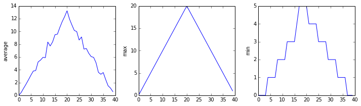

inflammation-02.csv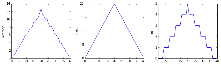

inflammation-03.csv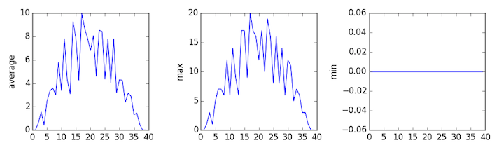

Sure enough, the maxima of the first two data sets show exactly the same ramp as the first, and their minima show the same staircase structure; a different situation has been revealed in the third dataset, where the maxima are a bit less regular, but the minima are consistently zero.

Making Choices

In our last lesson, we discovered something suspicious was going on in our inflammation data by drawing some plots. How can we use Python to automatically recognize the different features we saw, and take a different action for each? In this lesson, we'll learn how to write code that runs only when certain conditions are true.

Conditionals

We can ask Python to take different actions, depending on a condition, with an if statement:

num = 37
if num > 100:
    print 'greater'
else:
    print 'not greater'
print 'done'

not greater
done

The second line of this code uses the keyword if to tell Python that we want to make a choice. If the test that follows the if statement is true, the body of the if (i.e., the lines indented underneath it) are executed. If the test is false, the body of the else is executed instead. Only one or the other is ever executed:

Conditional statements don't have to include an else. If there isn't one, Python simply does nothing if the test is false:

num = 53
print 'before conditional...'
if num > 100:
    print '53 is greater than 100'
print '...after conditional'

before conditional...
...after conditional

We can also chain several tests together using elif, which is short for "else if". The following Python code uses elif to print the sign of a number.

num = -3

if num > 0:
    print num, "is positive"
elif num == 0:
    print num, "is zero"
else:
    print num, "is negative"

"-3 is negative"

One important thing to notice in the code above is that we use a double equals sign == to test for equality rather than a single equals sign because the latter is used to mean assignment.

We can also combine tests using and and or. and is only true if both parts are true:

if (1 > 0) and (-1 > 0):
    print 'both parts are true'
else:
    print 'one part is not true'

one part is not true

while or is true if at least one part is true:

if (1 < 0) or (-1 < 0):
    print 'at least one test is true'

at least one test is true

Checking our Data

Now that we've seen how conditionals work, we can use them to check for the suspicious features we saw in our inflammation data. In the first couple of plots, the maximum inflammation per day seemed to rise like a straight line, one unit per day. We can check for this inside the for loop we wrote with the following conditional:

if data.min(axis=0)[0] == 0 and data.max(axis=0)[20] == 20:
    print 'Suspicious looking maxima!'

We also saw a different problem in the third dataset; the minima per day were all zero (looks like a healthy person snuck into our study). We can also check for this with an elif condition:

elif data.min(axis=0).sum() == 0:
    print 'Minima add up to zero!'

And if neither of these conditions are true, we can use else to give the all-clear:

else:
    print 'Seems OK!'

Let's test that out:

data = numpy.loadtxt(fname='inflammation-01.csv', delimiter=',')
if data.max(axis=0)[0] == 0 and data.max(axis=0)[20] == 20:
    print 'Suspicious looking maxima!'
elif data.min(axis=0).sum() == 0:
    print 'Minima add up to zero!'
else:
    print 'Seems OK!'

Suspicious looking maxima!

data = numpy.loadtxt(fname='inflammation-03.csv', delimiter=',')
if data.max(axis=0)[0] == 0 and data.max(axis=0)[20] == 20:
    print 'Suspicious looking maxima!'
elif data.min(axis=0).sum() == 0:
    print 'Minima add up to zero!'
else:
    print 'Seems OK!'

Minima add up to zero!

In this way, we have asked Python to do something different depending on the condition of our data. Here we printed messages in all cases, but we could also imagine not using the else catch-all so that messages are only printed when something is wrong, freeing us from having to manually examine every plot for features we've seen before.

if 4 > 5:
    print 'A'
elif 4 == 5:
    print 'B'
elif 4 < 5:
    print 'C'

if '': print 'empty string is true'
if 'word': print 'word is true'
if []: print 'empty list is true'
if [1, 2, 3]: print 'non-empty list is true'
if 0: print 'zero is true'
if 1: print 'one is true'

x = 1  # original value
x += 1 # add one to x, assigning result back to x
x *= 3 # multiply x by 3
print x

6

left = 'L'
right = 'R'

temp = left
left = right
right = temp

left, right = right, left

Creating Functions

At this point, we've written code to draw some interesting features in our inflammation data, loop over all our data files to quickly draw these plots for each of them, and have Python make decisions based on what it sees in our data. But, our code is getting pretty long and complicated; what if we had thousands of datasets, and didn't want to generate a figure for every single one? Commenting out the figure-drawing code is a nuisance. Also, what if we want to use that code again, on a different dataset or at a different point in our program? Cutting and pasting it is going to make our code get very long and very repetative, very quickly. We'd like a way to package our code so that it is easier to reuse, and Python provides for this by letting us define things called 'functions' - a shorthand way of re-executing longer pieces of code.

Let's start by defining a function fahr_to_kelvin that converts temperatures from Fahrenheit to Kelvin:

def fahr_to_kelvin(temp):
    return ((temp - 32) * (5/9)) + 273.15

The function definition opens with the word def, which is followed by the name of the function and a parenthesized list of parameter names. The body of the function --- the statements that are executed when it runs --- is indented below the definition line, typically by four spaces.

When we call the function, the values we pass to it are assigned to those variables so that we can use them inside the function. Inside the function, we use a return statement to send a result back to whoever asked for it.

Let's try running our function. Calling our own function is no different from calling any other function:

print 'freezing point of water:', fahr_to_kelvin(32)
print 'boiling point of water:', fahr_to_kelvin(212)

freezing point of water: 273.15
boiling point of water: 273.15

We've successfully called the function that we defined, and we have access to the value that we returned. Unfortunately, the value returned doesn't look right. What went wrong?

Debugging a Function

Debugging is when we fix a piece of code that we know is working incorrectly. In this case, we know that fahr_to_kelvin is giving us the wrong answer, so let's find out why.

For big pieces of code, there are tools called debuggers that aid in this process. Since we just have a short function, we'll debug by choosing some parameter value, breaking our function into small parts, and printing out the value of each part.

# We'll use temp = 212, the boiling point of water, which was incorrect
print "212 - 32:", 212 - 32

212 - 32: 180

print "(212 - 32) * (5/9):", (212 - 32) * (5/9)

(212 - 32) * (5/9): 0

Aha! The problem comes when we multiply by 5/9. This is because 5/9 is actually 0.

5/9

0

Computers store numbers in one of two ways: as integers or as floating-point numbers (or floats). The first are the numbers we usually count with; the second have fractional parts. Addition, subtraction and multiplication work on both as we'd expect, but division works differently. If we divide one integer by another, we get the quotient without the remainder:

print '10/3 is:', 10/3

10/3 is: 3

If either part of the division is a float, on the other hand, the computer creates a floating-point answer:

print '10.0/3 is:', 10.0/3

10.0/3 is: 3.33333333333

The computer does this for historical reasons: integer operations were much faster on early machines, and this behavior is actually useful in a lot of situations. It's still confusing, though, so Python 3 produces a floating-point answer when dividing integers if it needs to. We're still using Python 2.7 in this class, though, so if we want 5/9 to give us the right answer, we have to write it as 5.0/9, 5/9.0, or some other variation.

Another way to create a floating-point answer is to explicitly tell the computer that you desire one. This is achieved by casting one of the numbers:

print 'float(10)/3 is:', float(10)/3

float(10)/3 is: 3.33333333333

The advantage to this method is it can be used with existing variables. Let's take a look:

a = 10
b = 3
print 'a/b is:', a/b
print 'float(a)/b is:', float(a)/b

a/b is: 3
float(a)/b is: 3.33333333333

Let's fix our fahr_to_kelvin function with this new knowledge:

def fahr_to_kelvin(temp):
    return ((temp - 32) * (5.0/9.0)) + 273.15

print 'freezing point of water:', fahr_to_kelvin(32)
print 'boiling point of water:', fahr_to_kelvin(212)

freezing point of water: 273.15
boiling point of water: 373.15

Composing Functions

Now that we've seen how to turn Fahrenheit into Kelvin, it's easy to turn Kelvin into Celsius:

def kelvin_to_celsius(temp):
    return temp - 273.15

print 'absolute zero in Celsius:', kelvin_to_celsius(0.0)

absolute zero in Celsius: -273.15

What about converting Fahrenheit to Celsius? We could write out the formula, but we don't need to. Instead, we can compose the two functions we have already created:

def fahr_to_celsius(temp):
    temp_k = fahr_to_kelvin(temp)
    result = kelvin_to_celsius(temp_k)
    return result

print 'freezing point of water in Celsius:', fahr_to_celsius(32.0)

freezing point of water in Celsius: 0.0

This is our first taste of how larger programs are built: we define basic operations, then combine them in ever-large chunks to get the effect we want. Real-life functions will usually be larger than the ones shown here --- typically half a dozen to a few dozen lines --- but they shouldn't ever be much longer than that, or the next person who reads it won't be able to understand what's going on.

Tidying up

Now that we know how to wrap bits of code up in functions, we can make our inflammation analyasis easier to read and easier to reuse. First, let's make an analyze function that generates our plots:

def analyze(filename):

    data = np.loadtxt(fname=filename, delimiter=',')

    fig = plt.figure(figsize=(10.0, 3.0))

    axes1 = fig.add_subplot(1, 3, 1)
    axes2 = fig.add_subplot(1, 3, 2)
    axes3 = fig.add_subplot(1, 3, 3)

    axes1.set_ylabel('average')
    axes1.plot(data.mean(axis=0))

    axes2.set_ylabel('max')
    axes2.plot(data.max(axis=0))

    axes3.set_ylabel('min')
    axes3.plot(data.min(axis=0))

    fig.tight_layout()
    plt.show(fig)

and another function called detect_problems that checks for those systematics we noticed:

def detect_problems(filename):

    data = np.loadtxt(fname=filename, delimiter=',')

    if data.max(axis=0)[0] == 0 and data.max(axis=0)[20] == 20:
        print 'Suspicious looking maxima!'
    elif data.min(axis=0).sum() == 0:
        print 'Minima add up to zero!'
    else:
        print 'Seems OK!'

Notice that rather than jumbling this code together in one giant for loop, we can now read and reuse both ideas separately. We can reproduce the previous analysis with a much simpler for loop:

for f in filenames[:3]:
    print f
    analyze(f)
    detect_problems(f)

By giving our functions human-readable names, we can more easily read and understand what is happening in the for loop. Even better, if at some later date we want to use either of those pieces of code again, we can do so in a single line.

Testing and Documenting

Once we start putting things in functions so that we can re-use them, we need to start testing that those functions are working correctly. To see how to do this, let's write a function to center a dataset around a particular value:

def center(data, desired):
    return (data - data.mean()) + desired

We could test this on our actual data, but since we don't know what the values ought to be, it will be hard to tell if the result was correct. Instead, let's use NumPy to create a matrix of 0's and then center that around 3:

z = numpy.zeros((2,2))
print center(z, 3)

[[ 3.  3.]
 [ 3.  3.]]

That looks right, so let's try center on our real data:

data = numpy.loadtxt(fname='inflammation-01.csv', delimiter=',')
print center(data, 0)

[[-6.14875 -6.14875 -5.14875 ..., -3.14875 -6.14875 -6.14875]
 [-6.14875 -5.14875 -4.14875 ..., -5.14875 -6.14875 -5.14875]
 [-6.14875 -5.14875 -5.14875 ..., -4.14875 -5.14875 -5.14875]
 ...,
 [-6.14875 -5.14875 -5.14875 ..., -5.14875 -5.14875 -5.14875]
 [-6.14875 -6.14875 -6.14875 ..., -6.14875 -4.14875 -6.14875]
 [-6.14875 -6.14875 -5.14875 ..., -5.14875 -5.14875 -6.14875]]

It's hard to tell from the default output whether the result is correct, but there are a few simple tests that will reassure us:

print 'original min, mean, and max are:', data.min(), data.mean(), data.max()
centered = center(data, 0)
print 'min, mean, and and max of centered data are:', centered.min(), centered.mean(), centered.max()

original min, mean, and max are: 0.0 6.14875 20.0
min, mean, and and max of centered data are: -6.14875 -3.49054118942e-15 13.85125

That seems almost right: the original mean was about 6.1, so the lower bound from zero is how about -6.1. The mean of the centered data isn't quite zero --- we'll explore why not in the challenges --- but it's pretty close. We can even go further and check that the standard deviation hasn't changed:

print 'std dev before and after:', data.std(), centered.std()

std dev before and after: 4.61383319712 4.61383319712

Those values look the same, but we probably wouldn't notice if they were different in the sixth decimal place. Let's do this instead:

print 'difference in standard deviations before and after:', data.std() - centered.std()

difference in standard deviations before and after: -3.5527136788e-15

Again, the difference is very small. It's still possible that our function is wrong, but it seems unlikely enough that we should probably get back to doing our analysis. We have one more task first, though: we should write some documentation for our function to remind ourselves later what it's for and how to use it.

The usual way to put documentation in software is to add comments like this:

# center(data, desired): return a new array containing the original data centered around the desired value.
def center(data, desired):
    return (data - data.mean()) + desired

There's a better way, though. If the first thing in a function is a string that isn't assigned to a variable, that string is attached to the function as its documentation:

def center(data, desired):
    '''Return a new array containing the original data centered around the desired value.'''
    return (data - data.mean()) + desired

This is better because we can now ask Python's built-in help system to show us the documentation for the function:

help(center)

Help on function center in module __main__:

center(data, desired)
    Return a new array containing the original data centered around the desired value.

A string like this is called a docstring. We don't need to use triple quotes when we write one, but if we do, we can break the string across multiple lines:

def center(data, desired):
    '''Return a new array containing the original data centered around the desired value.
    Example: center([1, 2, 3], 0) => [-1, 0, 1]'''
    return (data - data.mean()) + desired

help(center)

Help on function center in module __main__:

center(data, desired)
    Return a new array containing the original data centered around the desired value.
    Example: center([1, 2, 3], 0) => [-1, 0, 1]

Defining Defaults

We have passed parameters to functions in two ways: directly, as in type(data), and by name, as in numpy.loadtxt(fname='something.csv', delimiter=','). In fact, we can pass the filename to loadtxt without the fname=:

numpy.loadtxt('inflammation-01.csv', delimiter=',')

array([[ 0.,  0.,  1., ...,  3.,  0.,  0.],
       [ 0.,  1.,  2., ...,  1.,  0.,  1.],
       [ 0.,  1.,  1., ...,  2.,  1.,  1.],
       ...,
       [ 0.,  1.,  1., ...,  1.,  1.,  1.],
       [ 0.,  0.,  0., ...,  0.,  2.,  0.],
       [ 0.,  0.,  1., ...,  1.,  1.,  0.]])

but we still need to say delimiter=:

numpy.loadtxt('inflammation-01.csv', ',')

---------------------------------------------------------------------------
TypeError                                 Traceback (most recent call last)
<ipython-input-26-e3bc6cf4fd6a> in <module>()
----> 1 numpy.loadtxt('inflammation-01.csv', ',')

/Users/gwilson/anaconda/lib/python2.7/site-packages/numpy/lib/npyio.pyc in loadtxt(fname, dtype, comments, delimiter, converters, skiprows, usecols, unpack, ndmin)
    775     try:
    776         # Make sure we're dealing with a proper dtype
--> 777         dtype = np.dtype(dtype)
    778         defconv = _getconv(dtype)
    779

TypeError: data type "," not understood

To understand what's going on, and make our own functions easier to use, let's re-define our center function like this:

def center(data, desired=0.0):
    '''Return a new array containing the original data centered around the desired value (0 by default).
    Example: center([1, 2, 3], 0) => [-1, 0, 1]'''
    return (data - data.mean()) + desired

The key change is that the second parameter is now written desired=0.0 instead of just desired. If we call the function with two arguments, it works as it did before:

test_data = numpy.zeros((2, 2))
print center(test_data, 3)

[[ 3.  3.]
 [ 3.  3.]]

But we can also now call it with just one parameter, in which case desired is automatically assigned the default value of 0.0:

more_data = 5 + numpy.zeros((2, 2))
print 'data before centering:'
print more_data
print 'centered data:'
print center(more_data)

data before centering:
[[ 5.  5.]
 [ 5.  5.]]
centered data:
[[ 0.  0.]
 [ 0.  0.]]

This is handy: if we usually want a function to work one way, but occasionally need it to do something else, we can allow people to pass a parameter when they need to but provide a default to make the normal case easier. The example below shows how Python matches values to parameters:

def display(a=1, b=2, c=3):
    print 'a:', a, 'b:', b, 'c:', c

print 'no parameters:'
display()
print 'one parameter:'
display(55)
print 'two parameters:'
display(55, 66)

no parameters:
a: 1 b: 2 c: 3
one parameter:
a: 55 b: 2 c: 3
two parameters:
a: 55 b: 66 c: 3

As this example shows, parameters are matched up from left to right, and any that haven't been given a value explicitly get their default value. We can override this behavior by naming the value as we pass it in:

print 'only setting the value of c'
display(c=77)

only setting the value of c
a: 1 b: 2 c: 77

With that in hand, let's look at the help for numpy.loadtxt:

help(numpy.loadtxt)

Help on function loadtxt in module numpy.lib.npyio:

loadtxt(fname, dtype=<type 'float'>, comments='#', delimiter=None, converters=None, skiprows=0, usecols=None, unpack=False, ndmin=0)
    Load data from a text file.

    Each row in the text file must have the same number of values.

    Parameters
    ----------
    fname : file or str
        File, filename, or generator to read.  If the filename extension is
        ``.gz`` or ``.bz2``, the file is first decompressed. Note that
        generators should return byte strings for Python 3k.
    dtype : data-type, optional
        Data-type of the resulting array; default: float.  If this is a
        record data-type, the resulting array will be 1-dimensional, and
        each row will be interpreted as an element of the array.  In this
        case, the number of columns used must match the number of fields in
        the data-type.
    comments : str, optional
        The character used to indicate the start of a comment;
        default: '#'.
    delimiter : str, optional
        The string used to separate values.  By default, this is any
        whitespace.
    converters : dict, optional
        A dictionary mapping column number to a function that will convert
        that column to a float.  E.g., if column 0 is a date string:
        ``converters = {0: datestr2num}``.  Converters can also be used to
        provide a default value for missing data (but see also `genfromtxt`):
        ``converters = {3: lambda s: float(s.strip() or 0)}``.  Default: None.
    skiprows : int, optional
        Skip the first `skiprows` lines; default: 0.
    usecols : sequence, optional
        Which columns to read, with 0 being the first.  For example,
        ``usecols = (1,4,5)`` will extract the 2nd, 5th and 6th columns.
        The default, None, results in all columns being read.
    unpack : bool, optional
        If True, the returned array is transposed, so that arguments may be
        unpacked using ``x, y, z = loadtxt(...)``.  When used with a record
        data-type, arrays are returned for each field.  Default is False.
    ndmin : int, optional
        The returned array will have at least `ndmin` dimensions.
        Otherwise mono-dimensional axes will be squeezed.
        Legal values: 0 (default), 1 or 2.
        .. versionadded:: 1.6.0

    Returns
    -------
    out : ndarray
        Data read from the text file.

    See Also
    --------
    load, fromstring, fromregex
    genfromtxt : Load data with missing values handled as specified.
    scipy.io.loadmat : reads MATLAB data files

    Notes
    -----
    This function aims to be a fast reader for simply formatted files.  The
    `genfromtxt` function provides more sophisticated handling of, e.g.,
    lines with missing values.

    Examples
    --------
    >>> from StringIO import StringIO   # StringIO behaves like a file object
    >>> c = StringIO("0 1\n2 3")
    >>> np.loadtxt(c)
    array([[ 0.,  1.],
           [ 2.,  3.]])

    >>> d = StringIO("M 21 72\nF 35 58")
    >>> np.loadtxt(d, dtype={'names': ('gender', 'age', 'weight'),
    ...                      'formats': ('S1', 'i4', 'f4')})
    array([('M', 21, 72.0), ('F', 35, 58.0)],
          dtype=[('gender', '|S1'), ('age', '<i4'), ('weight', '<f4')])

    >>> c = StringIO("1,0,2\n3,0,4")
    >>> x, y = np.loadtxt(c, delimiter=',', usecols=(0, 2), unpack=True)
    >>> x
    array([ 1.,  3.])
    >>> y
    array([ 2.,  4.])

There's a lot of information here, but the most important part is the first couple of lines:

loadtxt(fname, dtype=<type 'float'>, comments='#', delimiter=None, converters=None, skiprows=0, usecols=None,
        unpack=False, ndmin=0)

This tells us that loadtxt has one parameter called fname that doesn't have a default value, and eight others that do. If we call the function like this:

numpy.loadtxt('inflammation-01.csv', ',')

then the filename is assigned to fname (which is what we want), but the delimiter string ',' is assigned to dtype rather than delimiter, because dtype is the second parameter in the list. However ',' isn't a known dtype so our code produced an error message when we tried to run it. When we call loadtxt we don't have to provide fname= for the filename because it's the first item in the list, but if we want the ',' to be assigned to the variable delimiter, we do have to provide delimiter= for the second parameter since delimiter is not the second parameter in the list.

print fence('name', '*')
*name*

print outer('helium')
hm

f = 0
k = 0

def f2k(f):
  k = ((f-32)*(5.0/9.0)) + 273.15
  return k

f2k(8)
f2k(41)
f2k(32)

print k

Errors and Exceptions

Every programmer encounters errors, both those who are just beginning, and those who have been programming for years. Encountering errors and exceptions can be very frustrating at times, and can make coding feel like a hopeless endeavour. However, understanding what the different types of errors are and when you are likely to encounter them can help a lot. Once you know why you get certain types of errors, they become much easier to fix.

Errors in Python have a very specific form, called a traceback. Let's examine one:

import errors_01
errors_01.favorite_ice_cream()

---------------------------------------------------------------------------
IndexError                                Traceback (most recent call last)
<ipython-input-1-9d0462a5b07c> in <module>()
      1 import errors_01
----> 2 errors_01.favorite_ice_cream()

/Users/jhamrick/project/swc/novice/python/errors_01.pyc in favorite_ice_cream()
      5         "strawberry"
      6     ]
----> 7     print ice_creams[3]

IndexError: list index out of range

This particular traceback has two levels. You can determine the number of levels by looking for the number of arrows on the left hand side. In this case:

1. The first shows code from the cell above, with an arrow pointing to Line 2 (which is favorite_ice_cream()).

2. The second shows some code in another function (favorite_ice_cream, located in the file errors_01.py), with an arrow pointing to Line 7 (which is print ice_creams[3]).

The last level is the actual place where the error occurred. The other level(s) show what function the program executed to get to the next level down. So, in this case, the program first performed a function call to the function favorite_ice_cream. Inside this function, the program encountered an error on Line 7, when it tried to run the code print ice_creams[3].

So what error did the program actually encounter? In the last line of the traceback, Python helpfully tells us the category or type of error (in this case, it is an IndexError) and a more detailed error message (in this case, it says "list index out of range").

If you encounter an error and don't know what it means, it is still important to read the traceback closely. That way, if you fix the error, but encounter a new one, you can tell that the error changed. Additionally, sometimes just knowing where the error occurred is enough to fix it, even if you don't entirely understand the message.

If you do encounter an error you don't recognize, try looking at the official documentation on errors. However, note that you may not always be able to find the error there, as it is possible to create custom errors. In that case, hopefully the custom error message is informative enough to help you figure out what went wrong.

Syntax Errors

When you forget a colon at the end of a line, accidentally add one space too many when indenting under an if statement, or forget a parentheses, you will encounter a syntax error. This means that Python couldn't figure out how to read your program. This is similar to forgetting punctuation in English:

this text is difficult to read there is no punctuation there is also no capitalization why is this hard because you have to figure out where each sentence ends you also have to figure out where each sentence begins to some extent it might be ambiguous if there should be a sentence break or not

People can typically figure out what is meant by text with no punctuation, but people are much smarter than computers. If Python doesn't know how to read the program, it will just give up and inform you with an error. For example:

def some_function()
    msg = "hello, world!"
    print msg
     return msg

  File "<ipython-input-3-6bb841ea1423>", line 1
    def some_function()
                       ^
SyntaxError: invalid syntax

Here, Python tells us that there is a SyntaxError on line 1, and even puts a little arrow in the place where there is an issue. In this case the problem is that the function definition is missing a colon at the end.

Actually, the function above has two issues with syntax. If we fix the problem with the colon, we see that there is also an IndentationError, which means that the lines in the function definition do not all have the same indentation:

def some_function():
    msg = "hello, world!"
    print msg
     return msg

  File "<ipython-input-4-ae290e7659cb>", line 4
    return msg
    ^
IndentationError: unexpected indent

Both SyntaxError and IndentationError indicate a problem with the syntax of your program, but an IndentationError is more specific: it always means that there is a problem with how your code is indented.

Variable Name Errors

Another very common type of error is called a NameError, and occurs when you try to use a variable that does not exist. For example:

print a

---------------------------------------------------------------------------
NameError                                 Traceback (most recent call last)
<ipython-input-7-9d7b17ad5387> in <module>()
----> 1 print a

NameError: name 'a' is not defined

Variable name errors come with some of the most informative error messages, which are usually of the form "name 'the_variable_name' is not defined".

Why does this error message occur? That's harder question to answer, because it depends on what your code is supposed to do. However, there are a few very common reasons why you might have an undefined variable. The first is that you meant to use a string, but forgot to put quotes around it:

print hello

---------------------------------------------------------------------------
NameError                                 Traceback (most recent call last)
<ipython-input-8-9553ee03b645> in <module>()
----> 1 print hello

NameError: name 'hello' is not defined

The second is that you just forgot to create the variable before using it. In the following example, count should have been defined (e.g., with count = 0) before the for loop:

for number in range(10):
    count = count + number
print "The count is: " + str(count)

---------------------------------------------------------------------------
NameError                                 Traceback (most recent call last)
<ipython-input-9-dd6a12d7ca5c> in <module>()
      1 for number in range(10):
----> 2     count = count + number
      3 print "The count is: " + str(count)

NameError: name 'count' is not defined

Finally, the third possibility is that you made a typo when you were writing your code. Let's say we fixed the error above by adding the line Count = 0 before the for loop. Frustratingly, this actually does not fix the error. Remember that variables are case-sensitive, so the variable count is different from Count. We still get the same error, because we still have not defined count:

Count = 0
for number in range(10):
    count = count + number
print "The count is: " + str(count)

---------------------------------------------------------------------------
NameError                                 Traceback (most recent call last)
<ipython-input-10-d77d40059aea> in <module>()
      1 Count = 0
      2 for number in range(10):
----> 3     count = count + number
      4 print "The count is: " + str(count)

NameError: name 'count' is not defined

Item Errors

Next up are errors having to do with containers (like lists and dictionaries) and the items within them. If you try to access an item in a list or a dictionary that does not exist, then you will get an error. This makes sense: if you asked someone what day they would like to get coffee, and they answered "caturday", you might be a bit annoyed. Python gets similarly annoyed if you try to ask it for an item that doesn't exist:

letters = ['a', 'b', 'c']
print "Letter #1 is " + letters[0]
print "Letter #2 is " + letters[1]
print "Letter #3 is " + letters[2]
print "Letter #4 is " + letters[3]

Letter #1 is a
Letter #2 is b
Letter #3 is c

---------------------------------------------------------------------------
IndexError                                Traceback (most recent call last)
<ipython-input-11-d817f55b7d6c> in <module>()
      3 print "Letter #2 is " + letters[1]
      4 print "Letter #3 is " + letters[2]
----> 5 print "Letter #4 is " + letters[3]

IndexError: list index out of range

Here, Python is telling us that there is an IndexError in our code, meaning we tried to access a list index that did not exist.

File Errors

The last type of error we'll cover today are those associated with reading and writing files: IOError. The "IO" in IOError stands for "input/output", which is just a fancy way of saying "reading/writing". If you try to read a file that does not exist, you will recieve an IOError telling you so. This is the most common reason why you would receive IOError, and if the error messages says "no such file or directory", then you know you have just tried to access a file that does not exist:

file_handle = open('myfile.txt', 'r')

---------------------------------------------------------------------------
IOError                                   Traceback (most recent call last)
<ipython-input-14-f6e1ac4aee96> in <module>()
----> 1 file_handle = open('myfile.txt', 'r')

IOError: [Errno 2] No such file or directory: 'myfile.txt'

One reason for receiving this error is that you specified an incorrect path to the file. For example, if I am currently in a folder called myproject, and I have a file in myproject/writing/myfile.txt, but I try to just open myfile.txt, this will fail. The correct path would be writing/myfile. xt. It is also possible (like with NameError) that you just made a typo.

Another issue could be that you used the "read" flag instead of the "write" flag. Python will not give you an error if you try to open a file for writing when the file does not exist. However, if you meant to open a file for reading, but accidentally opened it for writing, and then try to read from it, you will get an error telling you that the file was not opened for reading:

file_handle = open('myfile.txt', 'w')
file_handle.read()

---------------------------------------------------------------------------
IOError                                   Traceback (most recent call last)
<ipython-input-15-b846479bc61f> in <module>()
      1 file_handle = open('myfile.txt', 'w')
----> 2 file_handle.read()

IOError: File not open for reading

import errors_02
errors_02.print_friday_message()

---------------------------------------------------------------------------
KeyError                                  Traceback (most recent call last)
<ipython-input-2-e4c4cbafeeb5> in <module>()
      1 import errors_02
----> 2 errors_02.print_friday_message()

/Users/jhamrick/project/swc/novice/python/errors_02.py in print_friday_message()
     13
     14 def print_friday_message():
---> 15     print_message("Friday")

/Users/jhamrick/project/swc/novice/python/errors_02.py in print_message(day)
      9         "sunday": "Aw, the weekend is almost over."
     10     }
---> 11     print messages[day]
     12
     13

KeyError: 'Friday'

def another_function
  print "Syntax errors are annoying."
   print "But at least python tells us about them!"
  print "So they are usually not too hard to fix."

for number in range(10):
    # use a if the number is a multiple of 3, otherwise use b
    if (Number % 3) == 0:
        message = message + a
    else:
        message = message + "b"
print message

seasons = ['Spring', 'Summer', 'Fall', 'Winter']
print 'My favorite season is ', seasons[4]

Defensive Programming

Our previous lessons have introduced the basic tools of programming: variables and lists, file I/O, loops, conditionals, and functions. What they haven't done is show us how to tell whether a program is getting the right answer, and how to tell if it's still getting the right answer as we make changes to it.

To achieve that, we need to:

• Write programs that check their own operation.
• Write and run tests for widely-used functions.
• Make sure we know what "correct" actually means.

The good news is, doing these things will speed up our programming, not slow it down. As in real carpentry --- the kind done with lumber --- the time saved by measuring carefully before cutting a piece of wood is much greater than the time that measuring takes.

Assertions

The first step toward getting the right answers from our programs is to assume that mistakes will happen and to guard against them. This is called defensive programming, and the most common way to do it is to add assertions to our code so that it checks itself as it runs. An assertion is simply a statement that something must be true at a certain point in a program. When Python sees one, it evaluates the assertion's condition. If it's true, Python does nothing, but if it's false, Python halts the program immediately and prints the error message if one is provided. For example, this piece of code halts as soon as the loop encounters a value that isn't positive:

numbers = [1.5, 2.3, 0.7, -0.001, 4.4]
total = 0.0
for n in numbers:
    assert n > 0.0, 'Data should only contain positive values'
    total += n
print 'total is:', total

---------------------------------------------------------------------------
AssertionError                            Traceback (most recent call last)
<ipython-input-19-33d87ea29ae4> in <module>()
      2 total = 0.0
      3 for n in numbers:
----> 4     assert n > 0.0, 'Data should only contain positive values'
      5     total += n
      6 print 'total is:', total

AssertionError: Data should only contain positive values

Programs like the Firefox browser are full of assertions: 10-20% of the code they contain are there to check that the other 80-90% are working correctly. Broadly speaking, assertions fall into three categories:

• A precondition is something that must be true at the start of a function in order for it to work correctly.

• A postcondition is something that the function guarantees is true when it finishes.

• An invariant is something that is always true at a particular point inside a piece of code.

For example, suppose we are representing rectangles using a tuple of four coordinates (x0, y0, x1, y1), representing the lower left and upper right corners of the rectangle. In order to do some calculations, we need to normalize the rectangle so that the lower left corner is at the origin and the longest side is 1.0 units long. This function does that, but checks that its input is correctly formatted and that its result makes sense:

def normalize_rectangle(rect):
    '''Normalizes a rectangle so that it is at the origin and 1.0 units long on its longest axis.'''
    assert len(rect) == 4, 'Rectangles must contain 4 coordinates'
    x0, y0, x1, y1 = rect
    assert x0 < x1, 'Invalid X coordinates'
    assert y0 < y1, 'Invalid Y coordinates'

    dx = x1 - x0
    dy = y1 - y0
    if dx > dy:
        scaled = float(dx) / dy
        upper_x, upper_y = 1.0, scaled
    else:
        scaled = float(dx) / dy
        upper_x, upper_y = scaled, 1.0

    assert 0 < upper_x <= 1.0, 'Calculated upper X coordinate invalid'
    assert 0 < upper_y <= 1.0, 'Calculated upper Y coordinate invalid'

    return (0, 0, upper_x, upper_y)

The preconditions on lines 2, 4, and 5 catch invalid inputs:

print normalize_rectangle( (0.0, 1.0, 2.0) ) # missing the fourth coordinate

---------------------------------------------------------------------------
AssertionError                            Traceback (most recent call last)
<ipython-input-21-3a97b1dcab70> in <module>()
----> 1 print normalize_rectangle( (0.0, 1.0, 2.0) ) # missing the fourth coordinate

<ipython-input-20-408dc39f3915> in normalize_rectangle(rect)
      1 def normalize_rectangle(rect):
      2     '''Normalizes a rectangle so that it is at the origin and 1.0 units long on its longest axis.'''
----> 3     assert len(rect) == 4, 'Rectangles must contain 4 coordinates'
      4     x0, y0, x1, y1 = rect
      5     assert x0 < x1, 'Invalid X coordinates'

AssertionError: Rectangles must contain 4 coordinates

print normalize_rectangle( (4.0, 2.0, 1.0, 5.0) ) # X axis inverted

---------------------------------------------------------------------------
AssertionError                            Traceback (most recent call last)
<ipython-input-22-f05ae7878a45> in <module>()
----> 1 print normalize_rectangle( (4.0, 2.0, 1.0, 5.0) ) # X axis inverted

<ipython-input-20-408dc39f3915> in normalize_rectangle(rect)
      3     assert len(rect) == 4, 'Rectangles must contain 4 coordinates'
      4     x0, y0, x1, y1 = rect
----> 5     assert x0 < x1, 'Invalid X coordinates'
      6     assert y0 < y1, 'Invalid Y coordinates'
      7

AssertionError: Invalid X coordinates

The post-conditions help us catch bugs by telling us when our calculations cannot have been correct. For example, if we normalize a rectangle that is taller than it is wide everything seems OK:

print normalize_rectangle( (0.0, 0.0, 1.0, 5.0) )

(0, 0, 0.2, 1.0)

but if we normalize one that's wider than it is tall, the assertion is triggered:

print normalize_rectangle( (0.0, 0.0, 5.0, 1.0) )

---------------------------------------------------------------------------
AssertionError                            Traceback (most recent call last)
<ipython-input-24-5f0ef7954aeb> in <module>()
----> 1 print normalize_rectangle( (0.0, 0.0, 5.0, 1.0) )

<ipython-input-20-408dc39f3915> in normalize_rectangle(rect)
     16
     17     assert 0 < upper_x <= 1.0, 'Calculated upper X coordinate invalid'
---> 18     assert 0 < upper_y <= 1.0, 'Calculated upper Y coordinate invalid'
     19
     20     return (0, 0, upper_x, upper_y)

AssertionError: Calculated upper Y coordinate invalid

Re-reading our function, we realize that line 10 should divide dy by dx rather than dx by dy. (You can display line numbers by typing Ctrl-M, then L.) If we had left out the assertion at the end of the function, we would have created and returned something that had the right shape as a valid answer, but wasn't. Detecting and debugging that would almost certainly have taken more time in the long run than writing the assertion.

But assertions aren't just about catching errors: they also help people understand programs. Each assertion gives the person reading the program a chance to check (consciously or otherwise) that their understanding matches what the code is doing.

Most good programmers follow two rules when adding assertions to their code. The first is, fail early, fail often. The greater the distance between when and where an error occurs and when it's noticed, the harder the error will be to debug, so good code catches mistakes as early as possible.

The second rule is, turn bugs into assertions or tests. Whenever you fix a bug, write an assertion that catches the mistake should you make it again. If you made a mistake in a piece of code, the odds are good that you have made other mistakes nearby, or will make the same mistake (or a related one) the next time you change it. Writing assertions to check that you haven't regressed (i.e., haven't re-introduced an old problem) can save a lot of time in the long run, and helps to warn people who are reading the code (including your future self) that this bit is tricky.

Test-Driven Development

An assertion checks that something is true at a particular point in the program. The next step is to check the overall behavior of a piece of code, i.e., to make sure that it produces the right output when it's given a particular input. For example, suppose we need to find where two or more time series overlap. The range of each time series is represented as a pair of numbers, which are the time the interval started and ended. The output is the largest range that they all include:

Most novice programmers would solve this problem like this:

1. Write a function range_overlap.
2. Call it interactively on two or three different inputs.
3. If it produces the wrong answer, fix the function and re-run that test.

This clearly works --- after all, thousands of scientists are doing it right now --- but there's a better way:

1. Write a short function for each test.
2. Write a range_overlap function that should pass those tests.
3. If range_overlap produces any wrong answers, fix it and re-run the test functions.

Writing the tests before writing the function they exercise is called test-driven development (TDD). Its advocates believe it produces better code faster because:

1. If people write tests after writing the thing to be tested, they are subject to confirmation bias, i.e., they subconsciously write tests to show that their code is correct, rather than to find errors.
2. Writing tests helps programmers figure out what the function is actually supposed to do.

Here are three test functions for range_overlap:

assert range_overlap([ (0.0, 1.0) ]) == (0.0, 1.0)
assert range_overlap([ (2.0, 3.0), (2.0, 4.0) ]) == (2.0, 3.0)
assert range_overlap([ (0.0, 1.0), (0.0, 2.0), (-1.0, 1.0) ]) == (0.0, 1.0)

---------------------------------------------------------------------------
AssertionError                            Traceback (most recent call last)
<ipython-input-25-d8be150fbef6> in <module>()
----> 1 assert range_overlap([ (0.0, 1.0) ]) == (0.0, 1.0)
      2 assert range_overlap([ (2.0, 3.0), (2.0, 4.0) ]) == (2.0, 3.0)
      3 assert range_overlap([ (0.0, 1.0), (0.0, 2.0), (-1.0, 1.0) ]) == (0.0, 1.0)

AssertionError:

The error is actually reassuring: we haven't written range_overlap yet, so if the tests passed, it would be a sign that someone else had and that we were accidentally using their function.

And as a bonus of writing these tests, we've implicitly defined what our input and output look like: we expect a list of pairs as input, and produce a single pair as output.

Something important is missing, though. We don't have any tests for the case where the ranges don't overlap at all:

assert range_overlap([ (0.0, 1.0), (5.0, 6.0) ]) == ???

What should range_overlap do in this case: fail with an error message, produce a special value like (0.0, 0.0) to signal that there's no overlap, or something else? Any actual implementation of the function will do one of these things; writing the tests first helps us figure out which is best before we're emotionally invested in whatever we happened to write before we realized there was an issue.

And what about this case?

assert range_overlap([ (0.0, 1.0), (1.0, 2.0) ]) == ???

Do two segments that touch at their endpoints overlap or not? Mathematicians usually say "yes", but engineers usually say "no". The best answer is "whatever is most useful in the rest of our program", but again, any actual implementation of range_overlap is going to do something, and whatever it is ought to be consistent with what it does when there's no overlap at all.

Since we're planning to use the range this function returns as the X axis in a time series chart, we decide that:

1. every overlap has to have non-zero width, and
2. we will return the special value None when there's no overlap.

None is built into Python, and means "nothing here". (Other languages often call the equivalent value null or nil). With that decision made, we can finish writing our last two tests:

assert range_overlap([ (0.0, 1.0), (5.0, 6.0) ]) == None
assert range_overlap([ (0.0, 1.0), (1.0, 2.0) ]) == None

---------------------------------------------------------------------------
AssertionError                            Traceback (most recent call last)
<ipython-input-26-d877ef460ba2> in <module>()
----> 1 assert range_overlap([ (0.0, 1.0), (5.0, 6.0) ]) == None
      2 assert range_overlap([ (0.0, 1.0), (1.0, 2.0) ]) == None

AssertionError:

Again, we get an error because we haven't written our function, but we're now ready to do so:

def range_overlap(ranges):
    '''Return common overlap among a set of [low, high] ranges.'''
    lowest = 0.0
    highest = 1.0
    for (low, high) in ranges:
        lowest = max(lowest, low)
        highest = min(highest, high)
    return (lowest, highest)

(Take a moment to think about why we use max to raise lowest and min to lower highest). We'd now like to re-run our tests, but they're scattered across three different cells. To make running them easier, let's put them all in a function:

def test_range_overlap():
    assert range_overlap([ (0.0, 1.0), (5.0, 6.0) ]) == None
    assert range_overlap([ (0.0, 1.0), (1.0, 2.0) ]) == None
    assert range_overlap([ (0.0, 1.0) ]) == (0.0, 1.0)
    assert range_overlap([ (2.0, 3.0), (2.0, 4.0) ]) == (2.0, 3.0)
    assert range_overlap([ (0.0, 1.0), (0.0, 2.0), (-1.0, 1.0) ]) == (0.0, 1.0)

We can now test range_overlap with a single function call:

test_range_overlap()

---------------------------------------------------------------------------
AssertionError                            Traceback (most recent call last)
<ipython-input-29-cf9215c96457> in <module>()
----> 1 test_range_overlap()

<ipython-input-28-5d4cd6fd41d9> in test_range_overlap()
      1 def test_range_overlap():
----> 2     assert range_overlap([ (0.0, 1.0), (5.0, 6.0) ]) == None
      3     assert range_overlap([ (0.0, 1.0), (1.0, 2.0) ]) == None
      4     assert range_overlap([ (0.0, 1.0) ]) == (0.0, 1.0)
      5     assert range_overlap([ (2.0, 3.0), (2.0, 4.0) ]) == (2.0, 3.0)

AssertionError:

The first of the tests that was supposed to produce None fails, so we know there's something wrong with our function. What we don't know, though, is whether the other four tests passed or failed, because Python halted the program as soon as it spotted the first error. Still, some information is better than none, and if we trace the behavior of the function with that input, we realize that we're initializing lowest and highest to 0.0 and 1.0 respectively, regardless of the input values. This violates another important rule of programming: always initialize from data.

running([1, 2, 3, 4])

[1, 3, 6, 10]

running('abc')

['a', 'ab', 'abc']

def running(values):
    assert len(values) > 0
    result = [values[0]]
    for v in values[1:]:
        assert result[-1] >= 0
        result.append(result[-1] + v)
        assert result[-1] >= result[0]
    return result

Debugging

Once testing has uncovered problems, the next step is to fix them. Many novices do this by making more-or-less random changes to their code until it seems to produce the right answer, but that's very inefficient (and the result is usually only correct for the one case they're testing). The more experienced a programmer is, the more systematically they debug, and most follow some variation on the rules explained below.

Know What It's Supposed to Do

The first step in debugging something is to know what it's supposed to do. "My program doesn't work" isn't good enough: in order to diagnose and fix problems, we need to be able to tell correct output from incorrect. If we can write a test case for the failing case --- i.e., if we can assert that with these inputs, the function should produce that result --- then we're ready to start debugging. If we can't, then we need to figure out how we're going to know when we've fixed things.

But writing test cases for scientific software is frequently harder than writing test cases for commercial applications, because if we knew what the output of the scientific code was supposed to be, we wouldn't be running the software: we'd be writing up our results and moving on to the next program. In practice, scientists tend to do the following:

1. Test with simplified data. Before doing statistics on a real data set, we should try calculating statistics for a single record, for two identical records, for two records whose values are one step apart, or for some other case where we can calculate the right answer by hand.

2. Test a simplified case. If our program is supposed to simulate magnetic eddies in rapidly-rotating blobs of supercooled helium, our first test should be a blob of helium that isn't rotating, and isn't being subjected to any external electromagnetic fields. Similarly, if we're looking at the effects of climate change on speciation, our first test should hold temperature, precipitation, and other factors constant.

3. Compare to an oracle. A test oracle is something whose results are trusted, such as experimental data, an older program, or a human expert. We use to test oracles to determine if our new program produces the correct results. If we have a test oracle, we should store its output for particular cases so that we can compare it with our new results as often as we like without re-running that program.

4. Check conservation laws. Mass, energy, and other quantitites are conserved in physical systems, so they should be in programs as well. Similarly, if we are analyzing patient data, the number of records should either stay the same or decrease as we move from one analysis to the next (since we might throw away outliers or records with missing values). If "new" patients start appearing out of nowhere as we move through our pipeline, it's probably a sign that something is wrong.

5. Visualize. Data analysts frequently use simple visualizations to check both the science they're doing and the correctness of their code (just as we did in the opening lesson of this tutorial). This should only be used for debugging as a last resort, though, since it's very hard to compare two visualizations automatically.

Make It Fail Every Time

We can only debug something when it fails, so the second step is always to find a test case that makes it fail every time. The "every time" part is important because few things are more frustrating than debugging an intermittent problem: if we have to call a function a dozen times to get a single failure, the odds are good that we'll scroll past the failure when it actually occurs.

As part of this, it's always important to check that our code is "plugged in", i.e., that we're actually exercising the problem that we think we are. Every programmer has spent hours chasing a bug, only to realize that they were actually calling their code on the wrong data set or with the wrong configuration parameters, or are using the wrong version of the software entirely. Mistakes like these are particularly likely to happen when we're tired, frustrated, and up against a deadline, which is one of the reasons late-night (or overnight) coding sessions are almost never worthwhile.

Make It Fail Fast

If it takes 20 minutes for the bug to surface, we can only do three experiments an hour. That doesn't must mean we'll get less data in more time: we're also more likely to be distracted by other things as we wait for our program to fail, which means the time we are spending on the problem is less focused. It's therefore critical to make it fail fast.

As well as making the program fail fast in time, we want to make it fail fast in space, i.e., we want to localize the failure to the smallest possible region of code:

1. The smaller the gap between cause and effect, the easier the connection is to find. Many programmers therefore use a divide and conquer strategy to find bugs, i.e., if the output of a function is wrong, they check whether things are OK in the middle, then concentrate on either the first or second half, and so on.

2. N things can interact in N² different ways, so every line of code that isn't run as part of a test means more than one thing we don't need to worry about.

Change One Thing at a Time, For a Reason

Replacing random chunks of code is unlikely to do much good. (After all, if you got it wrong the first time, you'll probably get it wrong the second and third as well.) Good programmers therefore change one thing at a time, for a reason They are either trying to gather more information ("is the bug still there if we change the order of the loops?") or test a fix ("can we make the bug go away by sorting our data before processing it?").

Every time we make a change, however small, we should re-run our tests immediately, because the more things we change at once, the harder it is to know what's responsible for what (those N² interactions again). And we should re-run all of our tests: more than half of fixes made to code introduce (or re-introduce) bugs, so re-running all of our tests tells us whether we have regressed.

Keep Track of What You've Done

Good scientists keep track of what they've done so that they can reproduce their work, and so that they don't waste time repeating the same experiments or running ones whose results won't be interesting. Similarly, debugging works best when we keep track of what we've done and how well it worked. If we find ourselves asking, "Did left followed by right with an odd number of lines cause the crash? Or was it right followed by left? Or was I using an even number of lines?" then it's time to step away from the computer, take a deep breath, and start working more systematically.

Records are particularly useful when the time comes to ask for help. People are more likely to listen to us when we can explain clearly what we did, and we're better able to give them the information they need to be useful.

Be Humble

And speaking of help: if we can't find a bug in 10 minutes, we should be humble and ask for help. Just explaining the problem aloud is often useful, since hearing what we're thinking helps us spot inconsistencies and hidden assumptions.

Asking for help also helps alleviate confirmation bias. If we have just spent an hour writing a complicated program, we want it to work, so we're likely to keep telling ourselves why it should, rather than searching for the reason it doesn't. People who aren't emotionally invested in the code can be more objective, which is why they're often able to spot the simple mistakes we have overlooked.

Part of being humble is learning from our mistakes. Programmers tend to get the same things wrong over and over: either they don't understand the language and libraries they're working with, or their model of how things work is wrong. In either case, taking note of why the error occurred and checking for it next time quickly turns into not making the mistake at all.

And that is what makes us most productive in the long run. As the saying goes, A week of hard work can sometimes save you an hour of thought. If we train ourselves to avoid making some kinds of mistakes, to break our code into modular, testable chunks, and to turn every assumption (or mistake) into an assertion, it will actually take us less time to produce working programs, not more.

Command-Line Programs

The IPython Notebook and other interactive tools are great for prototyping code and exploring data, but sooner or later we will want to use our program in a pipeline or run it in a shell script to process thousands of data files. In order to do that, we need to make our programs work like other Unix command-line tools. For example, we may want a program that reads a dataset and prints the average inflammation per patient.

This program does exactly what we want - it prints the average inflammation per patient for a given file.

$ python readings.py --mean inflammation-01.csv
5.45
5.425
6.1
...
6.4
7.05
5.9

We might also want to look at the minimum of the first four lines

$ head -4 inflammation-01.csv | python readings.py --min

or the maximum inflammations in several files one after another:

$ python readings.py --max inflammation-*.csv

Our scripts should do the following:

1. If no filename is given on the command line, read data from standard input.
2. If one or more filenames are given, read data from them and report statistics for each file separately.
3. Use the --min, --mean, or --max flag to determine what statistic to print.

To make this work, we need to know how to handle command-line arguments in a program, and how to get at standard input. We'll tackle these questions in turn below.

Command-Line Arguments

Using the text editor of your choice, save the following in a text file called sys-version.py:

import sys
print 'version is', sys.version

The first line imports a library called sys, which is short for "system". It defines values such as sys.version, which describes which version of Python we are running. We can run this script from the command line like this:

$ python sys-version.py

version is 2.7.5 |Anaconda 1.8.0 (x86_64)| (default, Oct 24 2013, 07:02:20)
[GCC 4.0.1 (Apple Inc. build 5493)]

Create another file called argv-list.py and save the following text to it.

import sys
print 'sys.argv is', sys.argv

The strange name argv stands for "argument values". Whenever Python runs a program, it takes all of the values given on the command line and puts them in the list sys.argv so that the program can determine what they were. If we run this program with no arguments:

$ python argv-list.py

sys.argv is ['argv-list.py']

the only thing in the list is the full path to our script, which is always sys.argv[0]. If we run it with a few arguments, however:

$ python argv-list.py first second third

sys.argv is ['argv-list.py', 'first', 'second', 'third']

then Python adds each of those arguments to that magic list.

With this in hand, let's build a version of readings.py that always prints the per-patient mean of a single data file. The first step is to write a function that outlines our implementation, and a placeholder for the function that does the actual work. By convention this function is usually called main, though we can call it whatever we want:

$ cat readings-01.py

import sys
import numpy

def main():
    script = sys.argv[0]
    filename = sys.argv[1]
    data = numpy.loadtxt(filename, delimiter=',')
    for m in data.mean(axis=1):
        print m

This function gets the name of the script from sys.argv[0], because that's where it's always put, and the name of the file to process from sys.argv[1]. Here's a simple test:

$ python readings-01.py inflammation-01.csv

There is no output because we have defined a function, but haven't actually called it. Let's add a call to main:

$ cat readings-02.py

import sys
import numpy

def main():
    script = sys.argv[0]
    filename = sys.argv[1]
    data = numpy.loadtxt(filename, delimiter=',')
    for m in data.mean(axis=1):
        print m

main()

and run that:

$ python readings-02.py inflammation-01.csv

5.45
5.425
6.1
5.9
5.55
6.225
5.975
6.65
6.625
6.525
6.775
5.8
6.225
5.75
5.225
6.3
6.55
5.7
5.85
6.55
5.775
5.825
6.175
6.1
5.8
6.425
6.05
6.025
6.175
6.55
6.175
6.35
6.725
6.125
7.075
5.725
5.925
6.15
6.075
5.75
5.975
5.725
6.3
5.9
6.75
5.925
7.225
6.15
5.95
6.275
5.7
6.1
6.825
5.975
6.725
5.7
6.25
6.4
7.05
5.9

Handling Multiple Files

The next step is to teach our program how to handle multiple files. Since 60 lines of output per file is a lot to page through, we'll start by using three smaller files, each of which has three days of data for two patients:

$ ls small-*.csv

small-01.csv small-02.csv small-03.csv

$ cat small-01.csv

0,0,1
0,1,2

$ python readings-02.py small-01.csv

0.333333333333
1.0

Using small data files as input also allows us to check our results more easily: here, for example, we can see that our program is calculating the mean correctly for each line, whereas we were really taking it on faith before. This is yet another rule of programming: test the simple things first.

We want our program to process each file separately, so we need a loop that executes once for each filename. If we specify the files on the command line, the filenames will be in sys.argv, but we need to be careful: sys.argv[0] will always be the name of our script, rather than the name of a file. We also need to handle an unknown number of filenames, since our program could be run for any number of files.

The solution to both problems is to loop over the contents of sys.argv[1:]. The '1' tells Python to start the slice at location 1, so the program's name isn't included; since we've left off the upper bound, the slice runs to the end of the list, and includes all the filenames. Here's our changed program readings-03.py:

$ cat readings-03.py

import sys
import numpy

def main():
    script = sys.argv[0]
    for filename in sys.argv[1:]:
        data = numpy.loadtxt(filename, delimiter=',')
        for m in data.mean(axis=1):
            print m

main()

and here it is in action:

$ python readings-03.py small-01.csv small-02.csv

0.333333333333
1.0
13.6666666667
11.0

Handling Command-Line Flags

The next step is to teach our program to pay attention to the --min, --mean, and --max flags. These always appear before the names of the files, so we could just do this:

$ cat readings-04.py

import sys
import numpy

def main():
    script = sys.argv[0]
    action = sys.argv[1]
    filenames = sys.argv[2:]

    for f in filenames:
        data = numpy.loadtxt(f, delimiter=',')

        if action == '--min':
            values = data.min(axis=1)
        elif action == '--mean':
            values = data.mean(axis=1)
        elif action == '--max':
            values = data.max(axis=1)

        for m in values:
            print m

main()

This works:

$ python readings-04.py --max small-01.csv

1.0
2.0

but there are several things wrong with it:

1. main is too large to read comfortably.

2. If action isn't one of the three recognized flags, the program loads each file but does nothing with it (because none of the branches in the conditional match). Silent failures like this are always hard to debug.

This version pulls the processing of each file out of the loop into a function of its own. It also checks that action is one of the allowed flags before doing any processing, so that the program fails fast:

$ cat readings-05.py

import sys
import numpy

def main():
    script = sys.argv[0]
    action = sys.argv[1]
    filenames = sys.argv[2:]
    assert action in ['--min', '--mean', '--max'], \
           'Action is not one of --min, --mean, or --max: ' + action
    for f in filenames:
        process(f, action)

def process(filename, action):
    data = numpy.loadtxt(filename, delimiter=',')

    if action == '--min':
        values = data.min(axis=1)
    elif action == '--mean':
        values = data.mean(axis=1)
    elif action == '--max':
        values = data.max(axis=1)

    for m in values:
        print m

main()

This is four lines longer than its predecessor, but broken into more digestible chunks of 8 and 12 lines.

Python has a module named argparse that helps handle complex command-line flags. We will not cover this module in this lesson but you can go to Tshepang Lekhonkhobe's Argparse tutorial that is part of Python's Official Documentation.

Handling Standard Input

The next thing our program has to do is read data from standard input if no filenames are given so that we can put it in a pipeline, redirect input to it, and so on. Let's experiment in another script called count-stdin.py:

$ cat count-stdin.py

import sys

count = 0
for line in sys.stdin:
    count += 1

print count, 'lines in standard input'

This little program reads lines from a special "file" called sys.stdin, which is automatically connected to the program's standard input. We don't have to open it --- Python and the operating system take care of that when the program starts up --- but we can do almost anything with it that we could do to a regular file. Let's try running it as if it were a regular command-line program:

$ python count-stdin.py < small-01.csv

2 lines in standard input

A common mistake is to try to run something that reads from standard input like this:

$ count_stdin.py small-01.csv

i.e., to forget the < character that redirect the file to standard input. In this case, there's nothing in standard input, so the program waits at the start of the loop for someone to type something on the keyboard. Since there's no way for us to do this, our program is stuck, and we have to halt it using the Interrupt option from the Kernel menu in the Notebook.

We now need to rewrite the program so that it loads data from sys.stdin if no filenames are provided. Luckily, numpy.loadtxt can handle either a filename or an open file as its first parameter, so we don't actually need to change process. That leaves main:

$ cat readings-06.py

def main():
    script = sys.argv[0]
    action = sys.argv[1]
    filenames = sys.argv[2:]
    assert action in ['--min', '--mean', '--max'], \
           'Action is not one of --min, --mean, or --max: ' + action
    if len(filenames) == 0:
        process(sys.stdin, action)
    else:
        for f in filenames:
            process(f, action)

Let's try it out:

$ python readings-06.py --mean small-01.csv

0.333333333333
1.0

That's better. In fact, that's done: the program now does everything we set out to do.

$ python arith.py add 1 2

3

$ python arith.py subtract 3 4

-1

$ python my_ls.py py

left.py
right.py
zero.py

Reference

Analyzing Patient Data

• Import a library into a program using import libraryname.
• Use the numpy library to work with arrays in Python.
• Use variable = value to assign a value to a variable in order to record it in memory.
• Variables are created on demand whenever a value is assigned to them.
• Use print something to display the value of something.
• The expression array.shape gives the shape of an array.
• Use array[x, y] to select a single element from an array.
• Array indices start at 0, not 1.
• Use low:high to specify a slice that includes the indices from low to high-1.
• All the indexing and slicing that works on arrays also works on strings.
• Use # some kind of explanation to add comments to programs.
• Use array.mean(), array.max(), and array.min() to calculate simple statistics.
• Use array.mean(axis=0) or array.mean(axis=1) to calculate statistics across the specified axis.
• Use the pyplot library from matplotlib for creating simple visualizations.

Repeating Actions with Loops

• Use for variable in collection to process the elements of a collection one at a time.
• The body of a for loop must be indented.
• Use len(thing) to determine the length of something that contains other values.

Storing Multiple Values in Lists

• [value1, value2, value3, ...] creates a list.
• Lists are indexed and sliced in the same way as strings and arrays.
• Lists are mutable (i.e., their values can be changed in place).
• Strings are immutable (i.e., the characters in them cannot be changed).

Analyzing Data from Multiple Files

• Use glob.glob(pattern) to create a list of files whose names match a pattern.
• Use * in a pattern to match zero or more characters, and ? to match any single character.

Making Choices

• Use the ImageGrid class from the ipythonblocks library to create simple "images" made of colored blocks.
• Specify colors use (red, green, blue) triples, each component of which is an integer in the range 0..255.
• Use if condition to start a conditional statement, elif condition to provide additional tests, and else to provide a default.
• The bodies of the branches of conditional statements must be indented.
• Use == to test for equality.
• X and Y is only true if both X and Y are true.
• X or Y is true if either X or Y, or both, are true.
• Zero, the empty string, and the empty list are considered false; all other numbers, strings, and lists are considered true.
• Nest loops to operate on multi-dimensional data.
• Put code whose parameters change frequently in a function, then call it with different parameter values to customize its behavior.

Creating Functions

• Define a function using def name(...params...).
• The body of a function must be indented.
• Call a function using name(...values...).
• Numbers are stored as integers or floating-point numbers.
• Integer division produces the whole part of the answer (not the fractional part).
• Each time a function is called, a new stack frame is created on the call stack to hold its parameters and local variables.
• Python looks for variables in the current stack frame before looking for them at the top level.
• Use help(thing) to view help for something.
• Put docstrings in functions to provide help for that function.
• Specify default values for parameters when defining a function using name=value in the parameter list.
• Parameters can be passed by matching based on name, by position, or by omitting them (in which case the default value is used).

Errors and Exceptions

• Tracebacks can look intimidating, but they give us a lot of useful information about what went wrong in our program, including where the error occurred and what type of error it was.
• An error having to do with the "grammar" or syntax of the program is called a SyntaxError. If the issue has to do with how the code is indented, then it will be called an IndentationError.
• A NameError will occur if you use a variable that has not been defined (either because you meant to use quotes around a string, you forgot to define the variable, or you just made a typo).
• Containers like lists and dictionaries will generate errors if you try to access items in them that do not exist. For lists, this type of error is called an IndexError; for dictionaries, it is called a KeyError.
• Trying to read a file that does not exist will give you an IOError. Trying to read a file that is open for writing, or writing to a file that is open for reading, will also give you an IOError.

Defensive Programming

• Program defensively, i.e., assume that errors are going to arise, and write code to detect them when they do.
• Put assertions in programs to check their state as they run, and to help readers understand how those programs are supposed to work.
• Use preconditions to check that the inputs to a function are safe to use.
• Use postconditions to check that the output from a function is safe to use.
• Write tests before writing code in order to help determine exactly what that code is supposed to do.

Debugging

• Know what code is supposed to do before trying to debug it.
• Make it fail every time.
• Make it fail fast.
• Change one thing at a time, and for a reason.
• Keep track of what you've done.
• Be humble.

Command-Line Programs

• The sys library connects a Python program to the system it is running on.
• The list sys.argv contains the command-line arguments that a program was run with.
• Avoid silent failures.
• The "file" sys.stdin connects to a program's standard input.
• The "file" sys.stdout connects to a program's standard output.

Glossary

additive color model

A way to represent colors as the sum of contributions from primary colors such as red, green, and blue.

argument

A value given to a function or program when it runs. The term is often used interchangeably (and inconsistently) with parameter.

assertion

An expression which is supposed to be true at a particular point in a program. Programmers typically put assertions in their code to check for errors; if the assertion fails (i.e., if the expression evaluates as false), the program halts and produces an error message. See also: invariant, precondition, postcondition.

assign

To give a value a name by associating a variable with it.

body

(of a function): the statements that are executed when a function runs.

call stack

A data structure inside a running program that keeps track of active function calls.

case-insensitive

Treating text as if upper and lower case characters of the same letter were the same. See also: case-sensitive.

case-sensitive

Treating text as if upper and lower case characters of the same letter are different. See also: case-insensitive.

comment

A remark in a program that is intended to help human readers understand what is going on, but is ignored by the computer. Comments in Python, R, and the Unix shell start with a # character and run to the end of the line; comments in SQL start with --, and other languages have other conventions.

compose

To apply one function to the result of another, such as f(g(x)).

conditional statement

A statement in a program that might or might not be executed depending on whether a test is true or false.

comma-separated values

(CSV) A common textual representation for tables in which the values in each row are separated by commas.

default value

A value to use for a parameter if nothing is specified explicitly.

defensive programming

The practice of writing programs that check their own operation to catch errors as early as possible.

delimiter

A character or characters used to separate individual values, such as the commas between columns in a CSV file.

docstring

Short for "documentation string", this refers to textual documentation embedded in Python programs. Unlike comments, docstrings are preserved in the running program and can be examined in interactive sessions.

documentation

Human-language text written to explain what software does, how it works, or how to use it.

dotted notation

A two-part notation used in many programming languages in which thing.component refers to the component belonging to thing.

empty string

A character string containing no characters, often thought of as the "zero" of text.

encapsulation

The practice of hiding something's implementation details so that the rest of a program can worry about what it does rather than how it does it.

floating-point number

A number containing a fractional part and an exponent. See also: integer.

for loop

A loop that is executed once for each value in some kind of set, list, or range. See also: while loop.

function call

A use of a function in another piece of software.

immutable

Unchangeable. The value of immutable data cannot be altered after it has been created. See also: mutable.

import

To load a library into a program.

in-place operators

An operator such as += that provides a shorthand notation for the common case in which the variable being assigned to is also an operand on the right hand side of the assignment. For example, the statement x += 3 means the same thing as x = x + 3.

index

A subscript that specifies the location of a single value in a collection, such as a single pixel in an image.

inner loop

A loop that is inside another loop. See also: outer loop.

integer

A whole number, such as -12343. See also: floating-point number.

invariant

An expression whose value doesn't change during the execution of a program, typically used in an assertion. See also: precondition, postcondition.

library

A family of code units (functions, classes, variables) that implement a set of related tasks.

loop variable

The variable that keeps track of the progress of the loop.

member

A variable contained within an object.

method

A function which is tied to a particular object. Each of an object's methods typically implements one of the things it can do, or one of the questions it can answer.

object

A collection of conceptually related variables (members) and functions using those variables (methods).

outer loop

A loop that contains another loop. See also: inner loop.

parameter

A variable named in the function's declaration that is used to hold a value passed into the call. The term is often used interchangeably (and inconsistently) with argument.

pipe

A connection from the output of one program to the input of another. When two or more programs are connected in this way, they are called a "pipeline".

postcondition

A condition that a function (or other block of code) guarantees is true once it has finished running. Postconditions are often represented using assertions.

precondition

A condition that must be true in order for a function (or other block of code) to run correctly.

regression

To re-introduce a bug that was once fixed.

return statement

A statement that causes a function to stop executing and return a value to its caller immediately.

RGB

An additive model that represents colors as combinations of red, green, and blue. Each color's value is typically in the range 0..255 (i.e., a one-byte integer).

sequence

A collection of information that is presented in a specific order. For example, in Python, a string is a sequence of characters, while a list is a sequence of any variable.

shape

An array's dimensions, represented as a vector. For example, a 5×3 array's shape is (5,3).

silent failure

Failing without producing any warning messages. Silent failures are hard to detect and debug.

slice

A regular subsequence of a larger sequence, such as the first five elements or every second element.

stack frame

A data structure that provides storage for a function's local variables. Each time a function is called, a new stack frame is created and put on the top of the call stack. When the function returns, the stack frame is discarded.

standard input

A process's default input stream. In interactive command-line applications, it is typically connected to the keyboard; in a pipe, it receives data from the standard output of the preceding process.

standard output

A process's default output stream. In interactive command-line applications, data sent to standard output is displayed on the screen; in a pipe, it is passed to the standard input of the next process.

string

Short for "character string", a sequence of zero or more characters.

syntax error

A programming error that occurs when statements are in an order or contain characters not expected by the programming language.

test oracle

A program, device, data set, or human being against which the results of a test can be compared.

test-driven development

The practice of writing unit tests before writing the code they test.

traceback

The sequence of function calls that led to an error.

tuple

An immutable sequence of values.

type

The classification of something in a program (for example, the contents of a variable) as a kind of number (e.g. floating-point, integer), string, or something else.

type of error

Indicates the nature of an error in a program. For example, in Python, an IOError to problems with file input/output. See also: syntax error.

while loop

A loop that keeps executing as long as some condition is true. See also: for loop.

Discussion

Rules of Debugging

1. Fail early, fail often.
2. Always initialize from data.
3. Know what it's supposed to do.
4. Make it fail every time.
5. Make it fail fast.
6. Change one thing at a time, for a reason.
7. Keep track of what we've done.
8. Be humble.
9. Test the simple things first.

And remember, a week of hard work can sometimes save you an hour of thought.

The Call Stack

Let's take a closer look at what happens when we call fahr_to_celsius(32.0). To make things clearer, we'll start by putting the initial value 32.0 in a variable and store the final result in one as well:

original = 32.0
final = fahr_to_celsius(original)

The diagram below shows what memory looks like after the first line has been executed:

When we call fahr_to_celsius, Python doesn't create the variable temp right away. Instead, it creates something called a stack frame to keep track of the variables defined by fahr_to_kelvin. Initially, this stack frame only holds the value of temp:

When we call fahr_to_kelvin inside fahr_to_celsius, Python creates another stack frame to hold fahr_to_kelvin's variables:

It does this because there are now two variables in play called temp: the parameter to fahr_to_celsius, and the parameter to fahr_to_kelvin. Having two variables with the same name in the same part of the program would be ambiguous, so Python (and every other modern programming language) creates a new stack frame for each function call to keep that function's variables separate from those defined by other functions.

When the call to fahr_to_kelvin returns a value, Python throws away fahr_to_kelvin's stack frame and creates a new variable in the stack frame for fahr_to_celsius to hold the temperature in Kelvin:

It then calls kelvin_to_celsius, which means it creates a stack frame to hold that function's variables:

Once again, Python throws away that stack frame when kelvin_to_celsius is done and creates the variable result in the stack frame for fahr_to_celsius:

Finally, when fahr_to_celsius is done, Python throws away its stack frame and puts its result in a new variable called final that lives in the stack frame we started with:

This final stack frame is always there; it holds the variables we defined outside the functions in our code. What it doesn't hold is the variables that were in the various stack frames. If we try to get the value of temp after our functions have finished running, Python tells us that there's no such thing:

print 'final value of temp after all function calls:', temp

---------------------------------------------------------------------------
NameError                                 Traceback (most recent call last)
<ipython-input-12-ffd9b4dbd5f1> in <module>()
----> 1 print 'final value of temp after all function calls:', temp

NameError: name 'temp' is not defined

final value of temp after all function calls:

Why go to all this trouble? Well, here's a function called span that calculates the difference between the mininum and maximum values in an array:

import numpy

def span(a):
diff = a.max() - a.min()
return diff

data = numpy.loadtxt(fname='inflammation-01.csv', delimiter=',')
print 'span of data', span(data)

span of data 20.0

Notice that span assigns a value to a variable called diff. We might very well use a variable with the same name to hold data:

diff = numpy.loadtxt(fname='inflammation-01.csv', delimiter=',')
print 'span of data:', span(diff)

span of data: 20.0

We don't expect diff to have the value 20.0 after this function call, so the name diff cannot refer to the same thing inside span as it does in the main body of our program. And yes, we could probably choose a different name than diff in our main program in this case, but we don't want to have to read every line of NumPy to see what variable names its functions use before calling any of those functions, just in case they change the values of our variables.

The big idea here is encapsulation, and it's the key to writing correct, comprehensible programs. A function's job is to turn several operations into one so that we can think about a single function call instead of a dozen or a hundred statements each time we want to do something. That only works if functions don't interfere with each other; if they do, we have to pay attention to the details once again, which quickly overloads our short-term memory.

print outer(fence('carbon', '+'))

Image Grids

Let's start by creating some simple heat maps of our own using a library called ipythonblocks. The first step is to create our own "image":

from ipythonblocks import ImageGrid

Unlike the import statements we have seen earlier, this one doesn't load the entire ipythonblocks library. Instead, it just loads ImageGrid from that library, since that's the only thing we need (for now).

Once we have ImageGrid loaded, we can use it to create a very simple grid of colored cells:

grid = ImageGrid(5, 3)
grid.show()

Just like a NumPy array, an ImageGrid has some properties that hold information about it:

print 'grid width:', grid.width
print 'grid height:', grid.height
print 'grid lines on:', grid.lines_on

grid width: 5
grid height: 3
grid lines on: True

The obvious thing to do with a grid like this is color in its cells, but in order to do that, we need to know how computers represent color. The most common schemes are RGB, which is short for "red, green, blue". RGB is an additive color model: every shade is some combination of red, green, and blue intensities. We can think of these three values as being the axes in a cube:

RGB Color Cube

An RGB color is an example of a multi-part value: like a Cartesian coordinate, it is one thing with several parts. We can represent such a value in Python using a tuple, which we write using parentheses instead of the square brackets used for a list:

position = (12.3, 45.6)
print 'position is:', position
color = (10, 20, 30)
print 'color is:', color

position is: (12.3, 45.6)
color is: (10, 20, 30)

We can select elements from tuples using indexing, just as we do with lists and arrays:

print 'first element of color is:', color[0]

first element of color is: 10

Unlike lists and arrays, though, tuples cannot be changed after they are created --- in technical terms, they are immutable:

color[0] = 40
print 'first element of color after change:', color[0]

---------------------------------------------------------------------------
TypeError                                 Traceback (most recent call last)
<ipython-input-11-9c3dd30a4e52> in <module>()
----> 1 color[0] = 40
2 print 'first element of color after change:', color[0]

TypeError: 'tuple' object does not support item assignment

If a tuple represents an RGB color, its red, green, and blue components can take on values between 0 and 255. The upper bound may seem odd, but it's the largest number that can be represented in an 8-bit byte (i.e., 2⁸-1). This makes it easy for computers to manipulate colors, while providing fine enough gradations to fool most human eyes, most of the time.

Let's see what a few RGB colors actually look like:

row = ImageGrid(8, 1)
row[0, 0] = (0, 0, 0)   # no color => black
row[1, 0] = (255, 255, 255) # all colors => white
row[2, 0] = (255, 0, 0) # all red
row[3, 0] = (0, 255, 0) # all green
row[4, 0] = (0, 0, 255) # all blue
row[5, 0] = (255, 255, 0) # red and green
row[6, 0] = (255, 0, 255) # red and blue
row[7, 0] = (0, 255, 255) # green and blue
row.show()

Simple color values like (0,255,0) are easy enough to decipher with a bit of practice, but what color is (214,90,127)? To help us, ipythonblocks provides a function called show_color:

from ipythonblocks import show_color
show_color(214, 90, 127)

It also provides a table of standard colors:

from ipythonblocks import colors
c = ImageGrid(3, 2)
c[0, 0] = colors['Fuchsia']
c[0, 1] = colors['Salmon']
c[1, 0] = colors['Orchid']
c[1, 1] = colors['Lavender']
c[2, 0] = colors['LimeGreen']
c[2, 1] = colors['HotPink']
c.show()

bar = ImageGrid(10, 1)
for x in range(10):
    bar[x, 0] = (0, 0, ____)
bar.show()

Instructor's Guide

Legend

We are using a dataset with records on inflammation from patients following an arthritis treatment.

We make reference in the lesson that this data is somehow strange. It is strange because it is fabricated! The script used to generate the inflammation data is included as tools/gen_inflammation.py.

Overall

This lesson is written as an introduction to Python, but its real purpose is to introduce the single most important idea in programming: how to solve problems by building functions, each of which can fit in a programmer's working memory. In order to teach that, we must teach people a little about the mechanics of manipulating data with lists and file I/O so that their functions can do things they actually care about. Our teaching order tries to show practical uses of every idea as soon as it is introduced; instructors should resist the temptation to explain the "other 90%" of the language as well.

The final example asks them to build a command-line tool that works with the Unix pipe-and-filter model. We do this because it is a useful skill and because it helps learners see that the software they use isn't magical. Tools like grep might be more sophisticated than the programs our learners can write at this point in their careers, but it's crucial they realize this is a difference of scale rather than kind.

Explain that we use Python because:

• It's free.
• It has a lot of scientific libraries, and more are constantly being added.
• It has a large scientific user community.
• It's easier for novices to learn than most of the mature alternatives. (Software Carpentry originally used Perl; when we switched, we found that we could cover as much material in two days in Python as we'd covered in three days in Perl, and that retention was higher.)

We do not include instructions on running the IPython Notebook in the tutorial because we want to focus on the language rather than the tools. Instructors should, however, walk learners through some basic operations: * Launch from the command line with ipython notebook. * Create a new notebook. * Enter code or data in a cell and execute it. * Explain the difference between In[#] and Out[#].

Watching the instructor grow programs step by step is as helpful to learners as anything to do with Python. Resist the urge to update a single cell repeatedly (which is what you'd probably do in real life). Instead, clone the previous cell and write the update in the new copy so that learners have a complete record of how the program grew. Once you've done this, you can say, "Now why don't we just breaks things into small functions right from the start?"

The discussion of command-line scripts assumes that students understand standard I/O and building filters, which are covered in the lesson on the shell.

Frequently Argued Issues (FAI)

• import ... as ... syntax.

  This syntax is commonly used in the scientific Python community; it is explicitly recommended in documentation to import numpy as np and import matplotlib.pyplot as plt. Despite that, we have decided not to introduce aliasing imports in this novice lesson due to the additional cognitive load it puts on students, despite the typing that it saves. A good summary of arguments for and against can be found in PR #61.

  It is up to you as an individual instructor whether you want to introduce these aliases when you teach this lesson, but we encourage you to please read those arguments thoroughly before deciding one way or the other.

Analyzing Patient Data

Repeating Actions with Loops

Storing Multiple Values in Lists

Analyzing Data from Multiple Files

Making Choices

Creating Functions

Errors and Exceptions

Defensive Programming

Debugging

Command-Line Programs

Licenses

Instructional Material

All Software Carpentry instructional material is made available under the Creative Commons Attribution license. The following is a human-readable summary of (and not a substitute for) the full legal text of the CC BY 4.0 license.

You are free:

• to Share---copy and redistribute the material in any medium or format
• to Adapt---remix, transform, and build upon the material

for any purpose, even commercially.

The licensor cannot revoke these freedoms as long as you follow the license terms.

Under the following terms:

• Attribution---You must give appropriate credit (mentioning that your work is derived from work that is Copyright © Software Carpentry and, where practical, linking to http://software-carpentry.org/), provide a link to the license, and indicate if changes were made. You may do so in any reasonable manner, but not in any way that suggests the licensor endorses you or your use.

No additional restrictions---You may not apply legal terms or technological measures that legally restrict others from doing anything the license permits. With the understanding that:

Notices:

• You do not have to comply with the license for elements of the material in the public domain or where your use is permitted by an applicable exception or limitation.
• No warranties are given. The license may not give you all of the permissions necessary for your intended use. For example, other rights such as publicity, privacy, or moral rights may limit how you use the material.

Software

Except where otherwise noted, the example programs and other software provided by Software Carpentry are made available under the OSI-approved MIT license.

Permission is hereby granted, free of charge, to any person obtaining a copy of this software and associated documentation files (the "Software"), to deal in the Software without restriction, including without limitation the rights to use, copy, modify, merge, publish, distribute, sublicense, and/or sell copies of the Software, and to permit persons to whom the Software is furnished to do so, subject to the following conditions:

The above copyright notice and this permission notice shall be included in all copies or substantial portions of the Software.

THE SOFTWARE IS PROVIDED "AS IS", WITHOUT WARRANTY OF ANY KIND, EXPRESS OR IMPLIED, INCLUDING BUT NOT LIMITED TO THE WARRANTIES OF MERCHANTABILITY, FITNESS FOR A PARTICULAR PURPOSE AND NONINFRINGEMENT. IN NO EVENT SHALL THE AUTHORS OR COPYRIGHT HOLDERS BE LIABLE FOR ANY CLAIM, DAMAGES OR OTHER LIABILITY, WHETHER IN AN ACTION OF CONTRACT, TORT OR OTHERWISE, ARISING FROM, OUT OF OR IN CONNECTION WITH THE SOFTWARE OR THE USE OR OTHER DEALINGS IN THE SOFTWARE.

Trademark

"Software Carpentry" and the Software Carpentry logo are registered trademarks of NumFOCUS.